5 Review of Inferential Statistics

You may recall from your introductory statistics course that there is a distinction between descriptive statistics and inferential statistics. The difference between these two branches of statistics is that:

Descriptive statistics describes the data that we have collected. For example, we might ask what the average of the student GPAs in the GPA dataset is within the sample we have collected.
Inferential statistics tries to generalize our conclusions from the sample we have collected to the population from which we drew the sample.

So far we have just treated linear regression as a descriptive tool. We have found the best line that describes the data that we have collected; we have not attempted to say anything about the line that we would have gotten had we measured (say) every student’s GPA rather than just the GPAs of the 1000 students we happen to have sampled.

At first, it may seem like trying to make a statement about what would happen if we measured every student is impossible, given that we have only measured a relatively small subset of students. Surprisingly, it turns out to be relatively easy! The “only” catch is that to do this we need to have randomly sampled from the population of interest.

In this chapter, we will review the essential concepts from statistical inference necessary for performing inference in the context of regression. The main concepts we will review are:

What is a population and what are the parameters of that population?
What are probabilities and what does it mean for the sample to be randomly sampled?
What are estimators and how do we measure their precision and accuracy?
How do we test hypotheses about the population?
How do we quantify uncertainty about the parameters of the population using confidence intervals?

In your introductory statistics class, you should have covered many different statistical inference procedures, including: inference for a population mean, inference for paired data, inference for a proportion, and so forth. To keep things lean, in this chapter we will focus only on performing inference for a population mean.

5.1 Wage Data

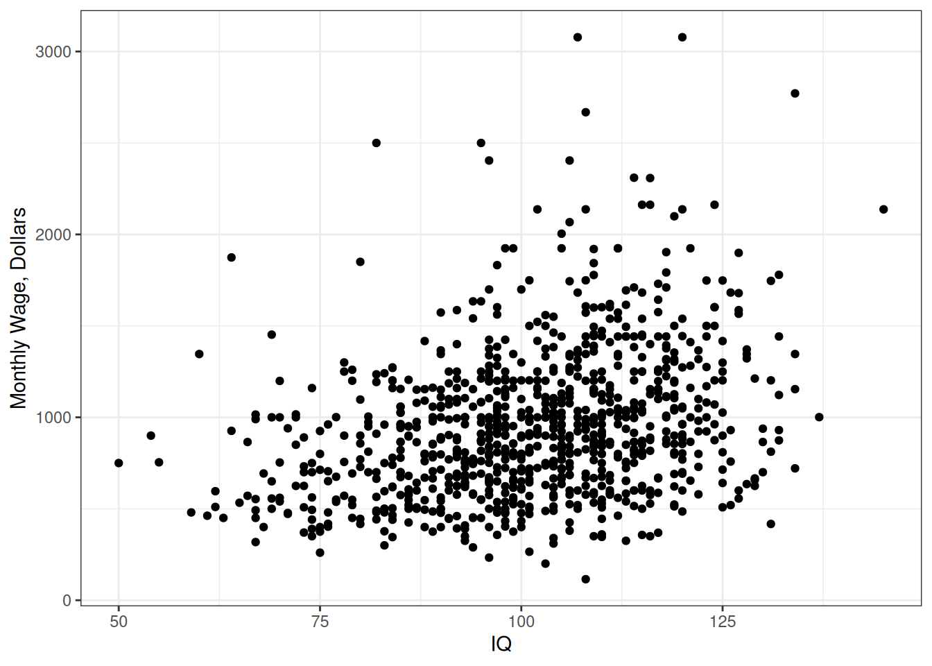
In this chapter, we will use the following dataset that consists of data from a survey of individuals, with the loose aim of predicting the monthly wages that an individual will earn:

filename <- "https://raw.githubusercontent.com/theodds/SDS-348/master/wages.csv"
wages <- read.csv(filename) %>% select(-X)
head(wages)

  wage hours  IQ educ exper tenure age married urban sibs birth.order
1  769    40  93   12    11      2  31     Yes   Yes    1           2
2  808    50 119   18    11     16  37     Yes   Yes    1          NA
3  825    40 108   14    11      9  33     Yes   Yes    1           2
4  650    40  96   12    13      7  32     Yes   Yes    4           3
5  562    40  74   11    14      5  34     Yes   Yes   10           6
6 1400    40 116   16    14      2  35     Yes   Yes    1           2
  mother.educ father.educ
1           8           8
2          14          14
3          14          14
4          12          12
5           6          11
6           8          NA

It consists of 935 individuals, and contains data only from 1980.¹

The wage that an individual earns will obviously depend on many factors, not all of which were (or even can be) measured. In this chapter, we will instead look at the measured IQ (intelligence quotient) scores in the sample. A plot of the relationship between IQ and wage is given below:

If you are unfamiliar with IQ tests, they are a tool to quantify the “general intelligence” of an individual, which is also what certain standardized tests that are used in college admissions attempt to do. On the high end, IQ tests can be used to track students into gifted learning programs; on the low end, they can be used to medically diagnose intellectual disabilities (under the DSM-5, a mild intellectual disability is associated with a measured IQ between 50 and 69 plus deficiencies in the ability to carry out everyday tasks). It is somewhat controversial as a measure of intelligence, and much has been written both for and against its use.

The reason we will analyze IQ in this chapter is that there is a lot of things that are known about it; specifically, it is constructed to have a normal distribution, with a mean o 100 and standard deviation of 15, when applied to randomly selected members of the general population. In this chapter we will attempt to answer the following question:

Question

Are the measured IQs in the sample we collected different than what we would expect to see in the general population? More specifically, does the population sampled from in this survey have a higher/lower IQ than the general population?

5.2 What is a Population?

To this point we have considered just fitting a line to the data we have collected, and computed quantities like the residual standard error and $R^2$ as different ways to quantify the performance of the model. This is all well and good if our only goal is to summarize the data we currently have, but we haven’t said anything about how to extend our conclusions to data that we do not (yet) have. That is, we need to be able to extend the conclusions we can draw from the sample to the entire population from which we collected our sample.

Borrowing from Danielle Navarro², we will adopt the following definition of a population:

(The population) refers to the set of all possible people, or all possible observations, that you want to draw conclusions about, and is generally much bigger than the sample. In an ideal world, the researcher would begin the study with a clear idea of what the population of interest is, since the process of designing a study and testing hypotheses about the data that it produces does depend on the population about which you want to make statements. However, that doesn’t always happen in practice: usually the researcher has a fairly vague idea of what the population is and designs the study as best he/she can on that basis.

To perform statistical inference we conceptualize the sample of data we collected as randomly chosen from the population - often this is assumed to be a simple random sample, where every member of the population has an equal chance of being selected. We can also make the further distinction between the sampling population (the population that we actually sampled from in collecting the data) and the target population (the population that we wished we had sampled from). In a perfect world these are the same population, but usually they are not.

In the context of the wages dataset, I might consider the following:

(Target) Population: the collection of all adults in the United States during the year 1980.
(Sample) Population: the collection of all adults who I might have asked to be in my survey, and who would have agreed to participate.

I do not actually know much about the survey design for the wages data, but usually for survey data these two populations are quite different: for example, in election polling there are often very big disagreements between what is predicted with a poll and what actually happens, due to the fact that most people ignore requests to participate in polls (what kind of weirdo actually responds to solicitations for a survey over the phone?).

5.2.1 Population Parameters

Population parameters are the attributes of the population that we are interested in. For example, for the wages dataset, we have made the claim that the average IQ should be 100 and the standard deviation should be 15 for the population of all individuals in the United States. We also asked whether the average is really 100 for the population of everybody who I could have tried to survey and who would have responded.

Again, the average IQ of the individuals that I really did sample, which is 101.28, is not a parameter. The only exception would be if I actually measured every possible person in the population. Instead, we think of the average IQ in the sample as an estimator of the population average. Later in the chapter, we will discuss how we can use estimators to draw conclusions about parameters.

5.3 Probabilities and Random Variables

To understand statistical inference, it is essential to first have some basic understanding of probabilities. We need probabilities to deal with the fact that the samples we collect are random: if we reran our survey or experiment, we would get different data. So, we can never be 100% certain that the sample we collected is representative of the broader population.

For the wages data, we ask the following question:

Does the fact the average IQ in the sample we collected is larger than 100 actually mean that we are sampling from a population with a higher IQ than average? Or is this just a quirk of the data that we happened to collect?

Because 101.28 is very close to 100, we might be inclined to believe that it is just a quirk of the data, but on the other hand the sample size of 935 is pretty large. In order to distinguish these possibilities, we will need to quantify things in terms of probabilities. Later in this chapter we will make the following statement:

We are 95% confident that the average IQ in the population sampled in the survey is between 100.31 and 102.25.

So it turns out that there is evidence that the average IQ in the population sampled is different from 100. But notice that this is a probabilistic statement! There is a chance that we are wrong, and the average is not between 100.31 and 102.25, with 95% representing our degree of confidence. If we require a higher degree of confidence, we will get a larger interval; for example, if we used 99.9% confidence instead, we would have gotten an interval of 99.66 to 102.90.

5.3.1 What is Probability?

In many real-world situations, we encounter uncertain outcomes, such as the result of a coin toss, the number of defective items in a manufacturing process, or the chance of rain on a given day. Our main use of probability will be to deal with uncertainties due to the use of a finite sample to draw inferences. To make informed decisions and predictions, we need a way to assign numerical values to these uncertainties. This is where probability comes into play.

Definition of Probability

Consider an experiment (such as conducting a survey of randomly selected people or flipping a coin) in which the outcome is uncertain. Then the probability of an event $A$, denoted by $\Pr(A)$, is the proportion of times that $A$ would occur if the experiment were independently repeated infinitely many times.

For example, if we toss a fair coin 1000 times and observed 498 heads, the observed frequency of heads would be 498 / 1000 = 0.498. The probability of observing heads is the limit of this fraction as the number of trials is increased towards infinity; if the coin is fair, then in the long run we should see 50% heads and 50% tails, so that $\Pr(\text{Heads is Flipped}) = 0.5$.

5.3.2 Random Variables

We will also frequently use the concept of a random variable, which is a numeric variable whose value is determined by the outcome of a random experiment.

Definition of a Random Variable

A random variable is a numeric summary of an experiment. It is typically denoted by an uppercase letter, such as $X$ or $Y$.

For example, for the wages data, the IQ of a randomly selected individual is an example of a random variable. By comparison, the sex of a randomly selected person is not a random variable, because it is not a number; it is possible to convert sex into a random variable by defining $X = 1$ if an individual’s sex is male and $X = 0$ otherwise.

As another example, let $X$ be the number of heads observed when flipping a fair coin three times. The possible values of $X$ are 0, 1, 2, and 3, each with a specific probability:

$\Pr(X = 0) = \frac{1}{8}$ (probability of getting 0 heads, only occurs if TTT)
$\Pr(X = 1) = \frac{3}{8}$ (probability of getting 1 head, occurs if TTH, THT, or HTT)
$\Pr(X = 2) = \frac{3}{8}$ (probability of getting 2 heads, occurs if THH, HTH, or HHT)
$\Pr(X = 3) = \frac{1}{8}$ (probability of getting 3 heads, occurs only if HHH)

Random variables are essential in probability theory and statistics because they allow us to model and analyze uncertain outcomes in a mathematical framework. By assigning probabilities to the possible values of a random variable, we can make predictions, talk about their averages, and assess the variability of the outcomes.

5.3.3 Types of Random Variables

Random variables can be classified into two main types: discrete and continuous.

Discrete random variables are random variables where the possible values can be listed out explicitly. Examples of discrete random variables that are included in the wages dataset include:

The sex of an individual, coded as $X = 1$ if male and $X = 0$ otherwise (the possible values are 0 and 1).
The number of siblings someone has (the possible values are 0, 1, 2, …).
The number of years of education that the individual’s mother has (the possible values are 0, 1, 2, …)

Notice that there does not need to be a finite number of possible values; it is enough just to be able to write them all out in a (potentially infinite) list³.

Continuous random variables are random variables that can take on any numeric values within a specified range or interval. In practice, variables that are truly continuous are rare (arguably non-existent) but we often treat variables that can take on a very large number of values in a given range as continuous. For the wages dataset this would include:

The IQ of an individual (can take any value larger than zero).
The wage of an individual (can take any value larger than zero).
The above two examples may give the impression that only “larger than zero” is allowed, but we can also have negative values (for example, the balance of someone’s bank account can be positive or negative) or values in a specific range (for example, the proportion of days that you have eggs for breakfast is between 0 and 1).

Continuous random variables can take an infinite number of possible values, at least theoretically⁴.

In this course, we will mainly be dealing with situations where the dependent variable is continuous, but will allow for both discrete and continuous independent variables. Time permitting, towards the end of the course we will discuss how to model discrete dependent variables.

5.3.4 What is a Probability Distribution?

The probability distribution of a random variable is a mathematical way to describe the likelihood of that random variable taking on different values.

Discrete random variables are associated with a probability mass function (PMF), which assigns a probability to each of the possible values that the random variable can take. For example, if $X = 1$ if a randomly selected individual is male and $X = 0$ otherwise, then (assuming 50% of all individuals are male) the PMF of $X$ is given by

\[ f_X(0) = \Pr(X = 0) = \frac{1}{2} \qquad \text{and} \qquad f_X(1) = \Pr(X = 1) = \frac{1}{2}. \]

Exercise

Suppose that we roll a fair six-sided die. What are the probability mass functions of the following quantities:

$X = 1$ if the outcome is divisible by 3 and $X = 0$ otherwise.
$X =$ the number on face-up side of the die.
$X =$ the square of the number on the face-up side of the die.

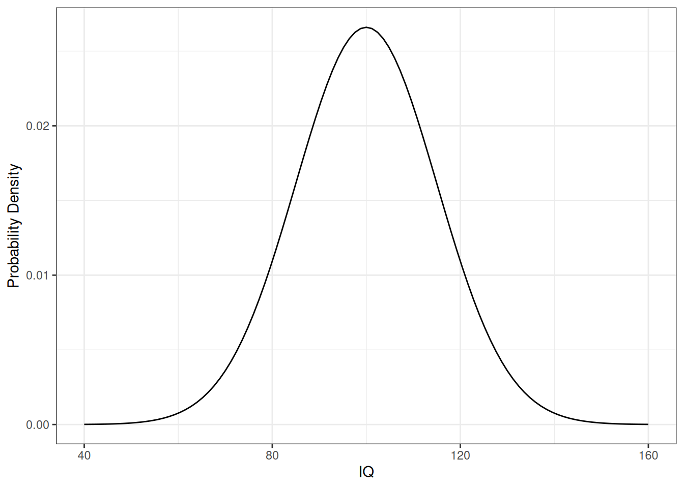
For continuous random variables, the probability distribution is instead represented by a probability density function (PDF). The PDF does not directly give the probability of a specific value occurring; instead, the PDF is used to calculate the probability of the random variable falling within a specific range of values. For example, IQs are usually associated with a normal distribution with mean $100$ and standard deviation $15$, which has a PDF that looks like this:

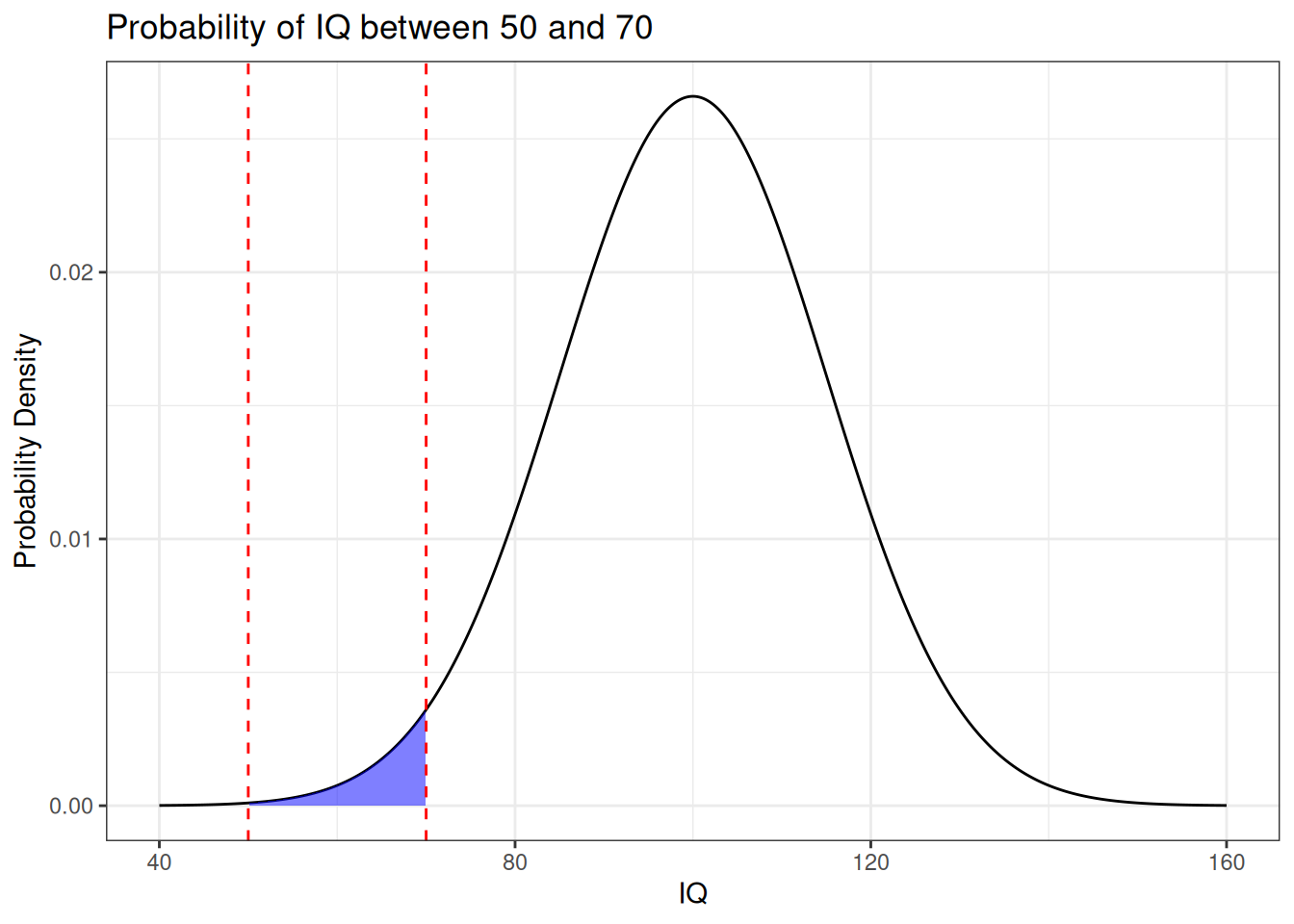
If we want to know the probability that a randomly selected individual has an IQ $X$ that is between 50 and 70, we can then look at the area under this curve between 50 and 70, like so:

This works out to approximately $0.022 \approx 2.2\%$.

In this class, the most important probability distributions we will look at are, in order of importance, the following:

The normal distribution.
Student’s $t$-distribution (or just the $t$-distribution).
The $F$-distribution.
If/when we discuss discrete dependent variables, the binomial and Poisson distributions.

The normal, $t$, and $F$ distributions are all continuous, while the binomial and Poisson distributions are discrete.

We will introduce these probability distributions as they are needed. In the case of the normal and $t$ distributions, that is right now!

5.3.5 The Normal Distribution

The normal distribution, also known as the Gaussian distribution, is arguably the most important probability distribution in all of statistics. It is a continuous distribution, and its PDF has a “bell shape”, with a peak at the average. It is also symmetric about the average, meaning that the curve to the left of the peak is a mirror image of the curve to the right of the peak.

The normal distribution is characterized by two population parameters:

The parameter $\mu$ represents the center or average of the distribution.
The parameter $\sigma$ represents the standard deviation of the distribution.

These two numbers completely pin down the normal distribution; if you tell me the mean and standard deviation of a distribution, and also tell me that it is a normal distribution, then I will know exactly what the distribution is.

The PDF of a Normal (Optional)

The normal distribution with mean $\mu$ and standard deviation $\sigma$ has a PDF with the following formula:

\[ f(x) = \frac{1}{\sqrt{2\pi \sigma^2}} e^{-\frac{(x - \mu)^2}{2 \sigma^2}}. \]

Mathematically, the probabilities associated to the normal distribution are integrals of $f(x)$, so for example the probability of an IQ being between 50 and 70 would be

\[ \int_{50}^{70} \frac{1}{\sqrt{2\pi \times 15^2}} e^{-\frac{(x - 100)^2}{2 \times 15^2}} \ dx. \]

This integral needs to be evaluated numerically, as there is no simple antiderivative of the normal PDF.

Some facts about the normal distribution that you might recall from your introductory statistics class include:

Symmetry: the normal distribution is symmetric about its mean, with 50% of the data falling on either side of the average. So, for example, 50% of IQs are less than 100 and 50% are greater than 100.
68-95-99.7 Rule Approximately 68% of the data, 95% of the data, and 99.7% of the data should fall within one, two, and three standard deviations of the mean, respectively. For example, 68% of individuals should have IQs between 85 and 115; 95% of individuals should have IQs between 70 and 130; and 99.7% of individuals should have IQs between 55 and 145.
Standardization: A normal distribution with a mean 0 and standard deviation 1 is called a standard normal distribution or a $Z$-distribution. We can always take a normal distribution and convert it to a standard normal distribution by subtracting the average and dividing by the standard deviation. For example

\[ \frac{\text{IQ} - 100}{15} \quad \text{has a standard normal distribution}. \]

Normality of Data is Usually An Assumption

In the above examples, I have just stated and assumed that IQs are “really” normally distributed with mean 100 and standard deviation 15. In the case of IQ, this is reasonable because psychologists get to define IQ and can force it to be true by design. In most cases, however, you have no control over whether your data is really normally distributed; another example of something that is assumed to be normally distributed is one’s height (after controlling for sex), but whether height really is or is not normally distributed can be disputed⁵.

There are two reasons that the normal distribution is so important in statistics:

The process of adding random numbers together tends to push the sum towards a normal distribution. This is known as the central limit theorem, and it is the basis of most of the statistical inference that we will do in this class. We will discuss the central limit theorem later in this chapter.
Sometimes the data itself will have a normal distribution. For example, in certain models in physics, there are physical quantities that have exactly a normal distribution, such as the velocity of a gas particle undergoing diffusion. There is usually no reason to expect this to be the case in, say, the social or biological sciences, but sometimes it happens.

Understanding the properties and characteristics of the normal distribution is crucial for many statistical techniques, including hypothesis testing, confidence intervals, and regression analysis, which we will explore further in this course.

5.3.6 The t-Distribution

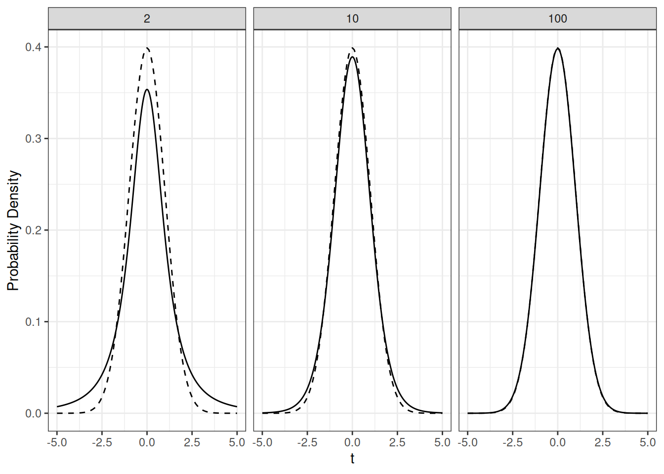
The $t$-distribution, also known as Student’s $t$-distribution, is another important continuous distribution in statistics. It is similar in shape to the standard normal distribution (the $Z$-distribution), but allows for more outliers. It is characterized by a single parameter $\nu$ called the degrees of freedom, which determines the shape of the distribution; as the degrees of freedom increase, the $t$-distribution approaches the $Z$-distribution, as illustrated below:

The solid graphs above represent the PDF of the $t$-distribution with 2, 10, and 100 degrees of freedom, while the dashed line presents the PDF of the standard normal distribution.

The $t$-distribution is important because, when our underlying data is normally distributed, it will describe the distribution of several important quantities that we will be looking at throughout the course. This makes it important when dealing with small sample sizes. The logic behind the use of the normal distribution and $t$-distribution in the problems we will look at is as follows:

When the sample size is large, many of the quantities we will be looking at will have, approximately, a standard normal distribution, irrespective of whether the original data was normal to begin with. This is a consequence of the central limit theorem.
When the sample size is small, we will no longer be able to appeal to the central limit theorem, so instead we can work with a $t$-distribution provided that the original data was normally distributed.
Because the $t$-distribution looks like a normal distribution when the sample size is large, it makes sense to just use the $t$-distribution 100% of the time without worrying about whether a $Z$-distribution or $t$-distribution is more appropriate.

Important applications of the $t$-distribution we will see include:

It is used when constructing confidence intervals for the population parameters we are interested in.
It is used for performing hypothesis tests about the population parameters we are interested in.
It will be used to make prediction intervals when forecasting future observations from the population (e.g., for the GPA dataset, if Alice is a new student we might want to make an interval such that we are 95% confident that Alice’s GPA will fall inside the interval).

Below, we will use the $t$-distribution to analyze the average IQ in the sampling population to see if it lines up with the hypothesized value of 100.

5.4 Estimating Population Parameters

For a given population parameter, and a sample from that population, our aim is usually to (i) construct an estimate of that parameter and (ii) quantify how precise our estimate of that parameter is. A quantity computed from the sample we actually have collected is called a statistic, while a statistic that has the purpose of estimating a population parameter is called an estimator. For example, the average IQ in our sample 101.28 is the usual estimator of the population average.

Below we discuss some common population parameters and their associated estimators, and then discuss how we evaluate these estimators.

5.4.1 Estimating the Population Average

First, we formally define the population average as follows.

Definition: The Population Average

For any random variable $Y$ we let $E(Y)$ denote the population average of this quantity; that is, $E(Y)$ is the average value of $Y$ we would observe if we sampled an infinite number of independent $Y$’s from the population and computed their average.

If $Y$ is discrete then $E(Y)$ can be calculated as

\[ E(Y) = \sum_y y \times f(y) \]

where $f(y)$ is the PMF of $Y$, and the sum is over all of the possible values of $Y$. Optional: If $Y$ is continuous, then $E(Y)$ can instead be calculated as

\[ E(Y) = \int_{-\infty}^\infty y \times f(y) \ dy \]

where $f(y)$ is the PDF of $Y$.

Example

Suppose that $Y$ is the face-up side of a fair six-sided die, so that $f(1) = f(2) = \cdots = f(6) = 1/6$. The expected value of $Y$ is then

\[ E(Y) = 1 \times \frac{1}{6} + 2 \times \frac{1}{6} + \cdots + 6 \times \frac{1}{6} = 3.5. \]

Exercise

Suppose that $Y$ is the face-up side of six-sided die, but now instead suppose that the die is not fair and instead we have

\[ \begin{aligned} f(1) = \frac{1}{21}, \qquad f(2) = \frac{2}{21}, \qquad f(3) = \frac{3}{21}, \\ f(4) = \frac{4}{21}, \qquad f(5) = \frac{5}{21}, \qquad f(6) = \frac{6}{21} \end{aligned} \]

What is the expected value of $Y$?

The population average is usually denoted with the Greek letter $\mu$.

The most common estimator of the population average is the sample average; that is, if $X_1, \ldots, X_N$ are sampled independently from the same population, we usually use the estimate

\[ \mu \approx \bar X = \frac{X_1 + \cdots + X_N}{N}. \]

We can estimate the population average IQ using the mean() function as follows:

mean(wages$IQ)

[1] 101.2824

We get the estimate of $\bar X = 101.28$ for $\mu$. This is pretty close to 100!

Population averages satisfy a couple of properties that make them quite easy to work with.

Properties of Population Averages

The population average of two random variables $Y$ and $Z$ is just the sum of the two population averages: $E(Y + Z) = E(Y) + E(Z)$.
If we multiply a random variable $Y$ by some number $k$ then the population average of the new quantity is $E(kY) = k \times E(Y)$.

5.4.2 Estimating the Population Standard Deviation and Variance

The population variance is defined similarly to the population average: it is the variance that we would get if we had access to the entire population, rather than a sample from the population. In math, it can be written as

\[ \text{Var}(X) = E\big([X - E(X)]^2\big) \]

so that it is the population average of the squared distance of $X$ from its population average. The population variance also has some useful properties:

Properties of the Population Variance

If $Y$ is a random variable and $k$ is some number, then:

$\text{Var}(Y + k) = \text{Var}(Y)$;
$\text{Var}(kY) = k^2 \, \text{Var}(Y)$;
$\text{Var}(X + Y) = \text{Var}(X) + \text{Var}(Y)$ provided that the random variables $X$ and $Y$ are independent (i.e., knowing the value of $X$ tells you nothing about $Y$, and vice versa).

The usual estimator of the population variance is the sample variance

\[ \text{Var}(X) \approx s^2 = \frac{(X_1 - \bar X)^2 + \cdots + (X_N - \bar X)^2}{N - 1}. \]

Similarly, the usual estimator of the population standard deviation is the sample standard deviation

\[ \text{SD}(X) \approx s = \sqrt{s^2}. \]

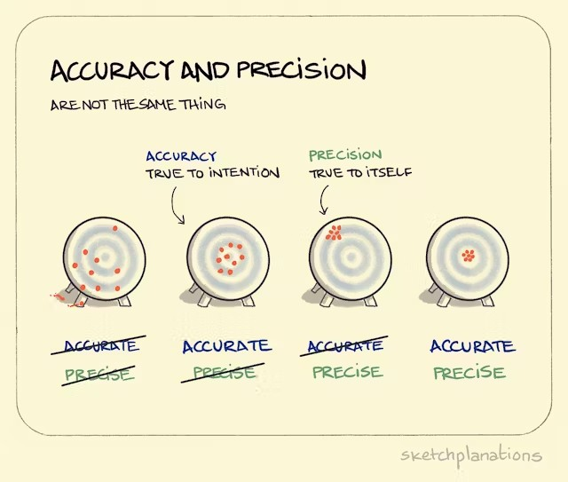
5.4.3 The Accuracy and Precision of an Estimator

When using a statistic or estimator to estimate a population parameter, it is important to consider both the precision of the estimator and its accuracy. The following figure illustrates the overall concept of accuracy and precision by analogy with throwing darts:

Borrowed with permission from https://sketchplanations.com/accuracy-and-precision

Ideally, we would like an estimator that is both accurate and precise. To make things a little bit more formal, we will introduce the bias of an estimator and its standard error.

The Bias of an Estimator

Consider an estimator $\widehat \theta$ of some population parameter $\theta$; for example, we could have $\theta$ equal to the population mean and $\widehat \theta$ equal to the sample mean, or $\theta$ equal to the population standard deviation and $\widehat \theta$ equal to the sample standard deviation.

Then, the bias of $\widehat \theta$ is how far off, on average, $\widehat \theta$ is from $\theta$; that is,

\[ \text{Bias}(\widehat \theta) = E(\widehat\theta) - \theta. \]

The Bias of Common Estimators

The usual estimate of the population mean $\mu$ is the sample mean $\bar X$. It turns out that $\bar X$ is unbiased, so that $E(\bar X) = \mu$.
The usual estimate of the population variance $\sigma^2 = \text{Var}(X)$ is the sample variance $s^2$. This estimator is also unbiased, so $E(s^2) = \sigma^2$. Notably, this would not be true if we used the denominator $N$ instead of $N - 1$ in the sample variance.
The usual estimator of the population standard deviation $\sigma$ is the sample standard deviation $s$. This estimator is biased, as it is systematically too small. There do not exist any unbiased estimators of $\sigma$, but the bias of $s$ is usually small (and gets closer and closer to unbiased as the sample size increases).

Good estimators are unbiased or at least have bias that goes to $0$ as $N$ increases. To go along with the bias of an estimator, we use the standard error of an estimator to quantify its precision.

The Precision of an Estimator

The standard error of $\widehat \theta$ is its standard deviation, so that

\[ \text{std. error}(\widehat \theta) = \sqrt{\text{Var}(\widehat \theta)} \]

When the variance of $\widehat \theta$ is not known, we will also use the term “standard error” to refer to any estimate of its standard deviation.

Why invent a new term to refer to the standard deviation? Frankly, I’m not really sure, aside from the fact that the term “standard error” gives us the vibe that we are estimating something, and are interested in quantifying how far off our estimate should be.

Standard Errors of Common Estimators

The standard error of $\bar X$ is $\frac{\sigma}{\sqrt N}$ or, when $\sigma$ is unknown, $\frac{s}{\sqrt N}$.
None of the other estimators we have looked at have simple standard errors, but the least squares estimators we learned about in the previous chapter do have simple standard errors. We will learn about these in the next chapter.

An estimator with a small standard error is considered precise. Typically, we expect that the larger our sample size the more precise our estimates will be; for example, the standard error of $\bar X$ is $\frac{\sigma}{\sqrt N}$, which gets smaller as $N$ gets larger.

In the context of the wages dataset, the sample mean of the IQ scores is unbiased and is relatively precise. Specifically, the standard error is

sd(wages$IQ) / sqrt(935)

[1] 0.4922738

So we expect our estimate of the population average IQ to be off by roughly 0.49 IQ points, on average.

5.4.4 Standardized Statistics and the Central Limit Theorem

Often in statistics we work with standardized statistics. The reason for this that standardized statistics are often close to a standard normal distribution due to a powerful result called the central limit theorem. The fact that we know that a standardized statistic has a normal distribution will be very useful when we start performing hypothesis tests and making confidence intervals.

Definition: Standardized Statistic

A standardized statistic (also known as a $Z$-score or $T$-score, depending on the context) is a statistic that has been rescaled by subtracting the quantity it is estimating and dividing by its standard error; that is, if $\widehat \theta$ is an estimator of $\theta$ with a standard error $s_{\widehat \theta}$ then the standardized version of $\widehat \theta$ is given by

\[ Z = \frac{\widehat \theta - \theta}{s_{\widehat \theta}}. \]

Example

If $X_1, \ldots, X_N$ are sampled from some population with mean $\mu$ and variance $\sigma^2$ then the usual estimator of $\mu$ is $\bar X$, which has a standard error of $\frac{s}{\sqrt N}$. Therefore, the standardized version of $\bar X$ is

\[ Z = \frac{\bar X - \mu}{s / \sqrt N}. \]

The central limit theorem states that, under certain conditions, standardized statistics will have approximately a standard normal distribution. In your introductory statistics class you learned this fact about $\bar X$ but it is actually true in many other contexts as well. For example, it is also true of $\widehat \beta_0$ and $\widehat \beta_1$ in simple linear regression. The version of the central limit theorem you learned about in your introductory statistics class is probably the following:

The Central Limit Theorem

Let $X_1, X_2, \ldots, X_N$ be a sequence of independent and identically distributed random variables with mean $\mu$ and variance $\sigma^2$. Let $\bar{X}_N$ be the sample mean of these variables. Then, as $N$ approaches infinity, the distribution of the standardized sample mean $Z = (\bar X - \mu) / (\sigma / \sqrt N)$ converges to the standard normal distribution. This result remains true if $\sigma$ is replaced with the sample standard deviation $s$.

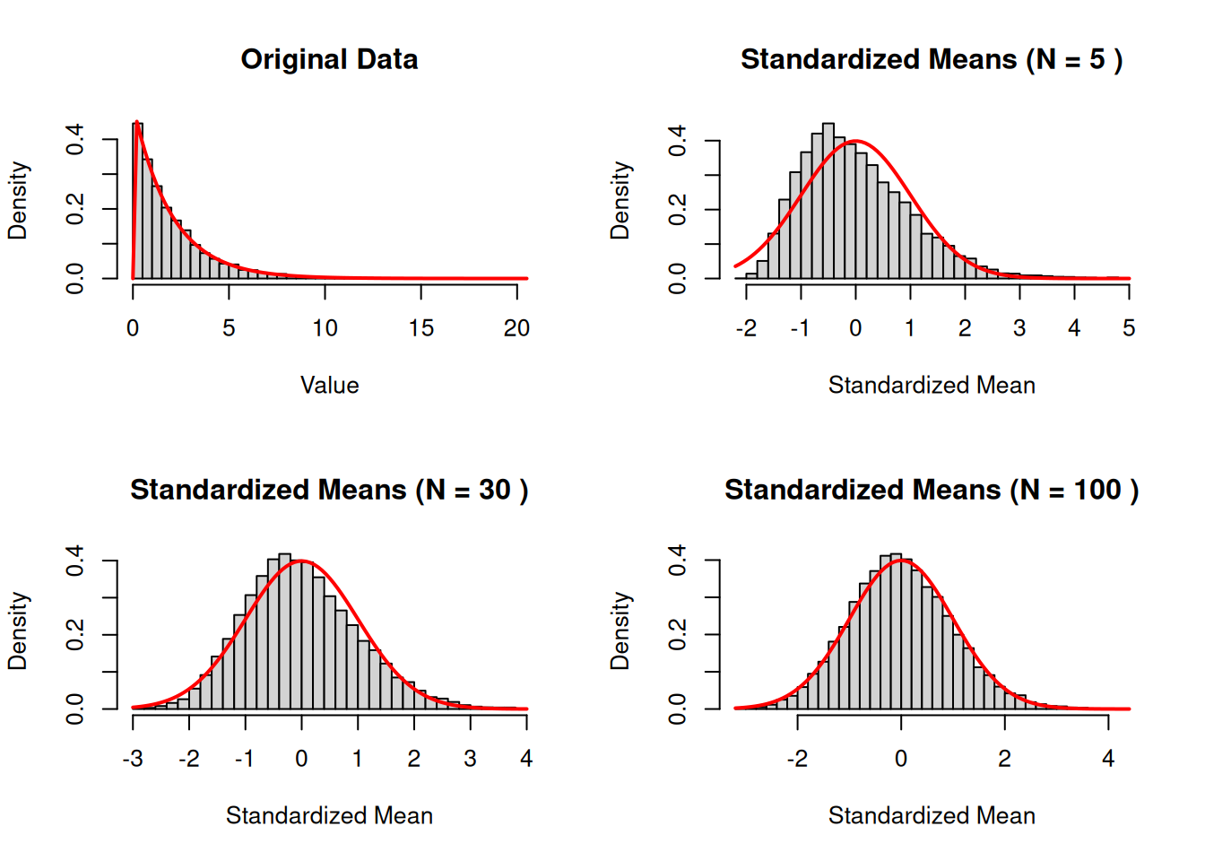
The central limit theorem is important because it can be used to draw inference about the population mean $\mu$ without making strong assumptions about the data. Below we show how the central limit theorem applies: from the original data (which is not normally distributed) we look at the distribution of the standardized average for larger and larger values of the sample size $N$. By the time we get to a sample size of $N = 30$, the standardized mean appears very close to a standard normal distribution.

The $t$-distribution also arises with standardized statistics, but works even if the sample size is not large.

The $t$-distribution

Let $X_1, X_2, \ldots, X_N$ be a sequence of independent normally distributed random variables with mean $\mu$ and variance $\sigma^2$. Let $\bar{X}$ be the sample mean of these variables. Then the standardized statistic

\[ T = \frac{\bar X - \mu}{s / \sqrt N} \]

has a $t$-distribution with $N - 1$ degrees of freedom.

The benefit of using the $t$-distribution is that it works even if the sample size is small. Again, we will see that this sort of thing is also true of the least squares coefficients provided that the underlying data are normally distributed.

What Do I Do?

In this class, we will use the following guidelines. TLDR: just use the $t$-distribution, regardless of the sample size or whether the data is actually normal or not.

In small samples, if the data is normally distributed, using the $t$-distribution for inferences is the right thing to do.
In large samples, if the data is normally distributed, using the $t$-distribution is still the right thing to do.
In large samples, if the data is not normally distributed, the central limit theorem applies and so we could use a $Z$-distribution if we wanted. But, because the $t$-distribution is basically the same thing in large samples, you should still just use the $t$-distribution, as it is usually slightly better even as an approximation than the $Z$-distribution. So, using the $t$-distribution is still the right thing to do.
In small samples, if the data is not normally distributed, there is no “right thing to do”, but it is definitely preferable to use the $t$-distribution in this case as well. Unless the data highly and obviously skewed and has a bunch of outliers, the $t$-distribution can still work pretty well as an approximation, while the $Z$-distribution might not. So, of the two options, using the $t$-distribution is the “least wrong” thing to do.

The alternative to using the $t$-distribution when the data is not normal that is often recommended is to use a “nonparametric” method. We will not use nonparametric methods in this course.

In the context of the wages dataset, we can look at the standardized version of the mean by subtracting the hypothesized average (100) and dividing by its standard error $(s / \sqrt N)$ to get

t_stat <- (mean(wages$IQ) - 100) / (sd(wages$IQ) / sqrt(935))
print(t_stat)

[1] 2.604958

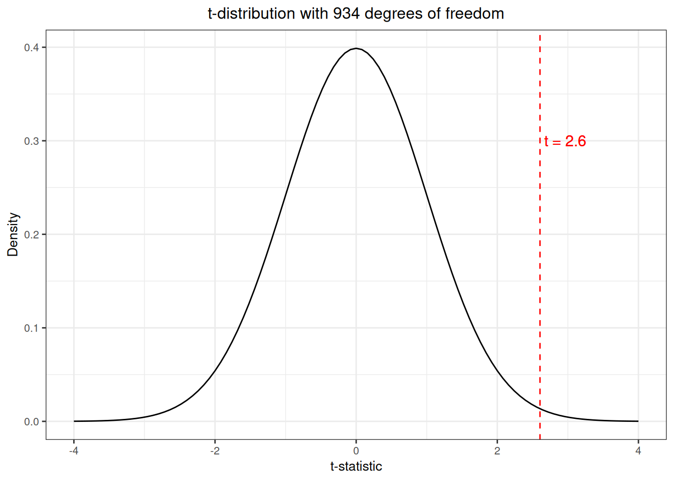
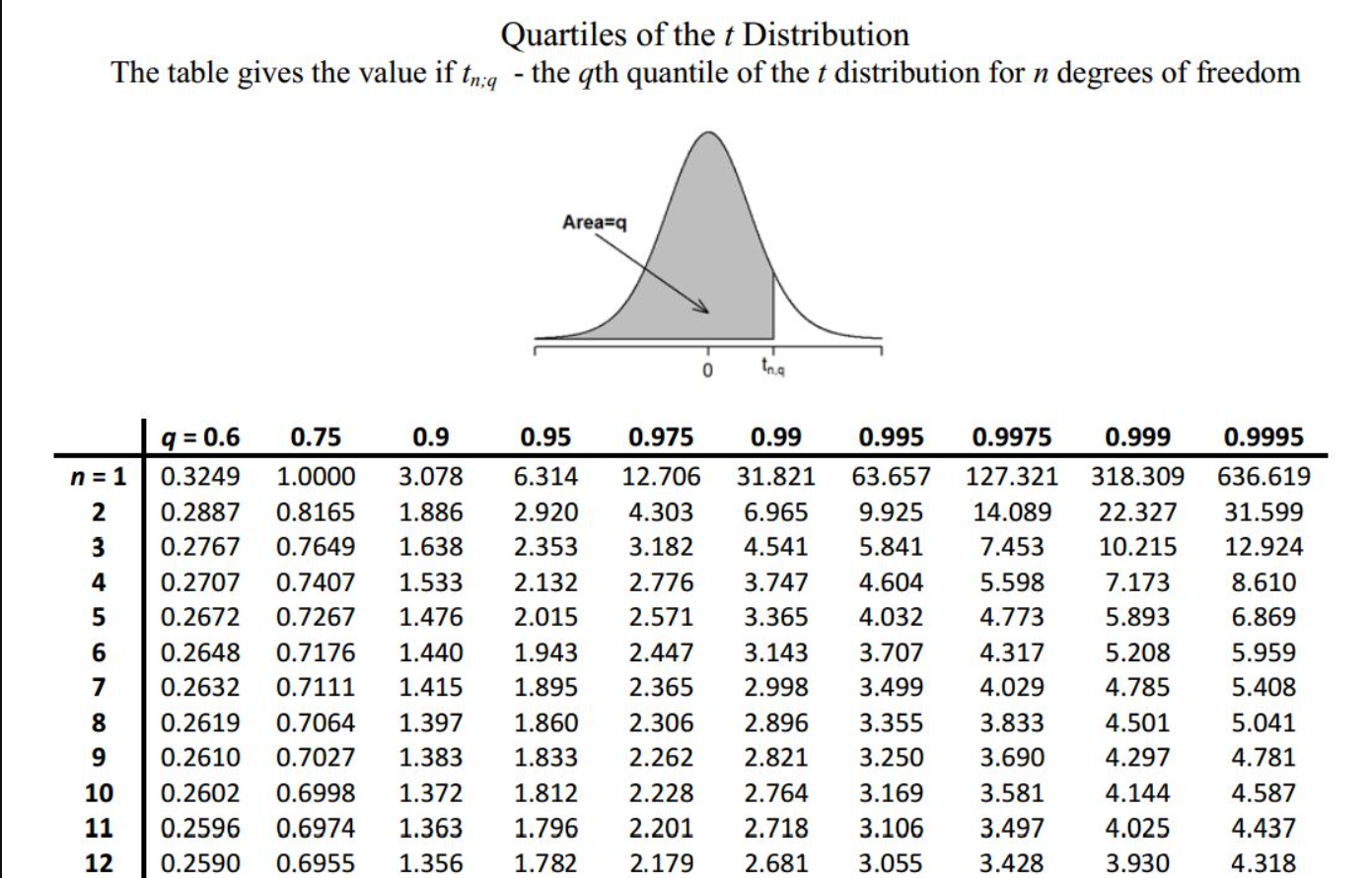
Question: is this value of the $T$-statistic weird? We were interested in testing whether the population average of $100$ was actually correct; if this was actually the case should we have expected to see a value of $T$ that is this large? Let’s take a closer look by comparing with the $t$-distribution with 934 degrees of freedom:

This value actually looks pretty unusual, sitting well out in the “tails” of the $T$-distribution! In the following section, we will discuss the problem of hypothesis testing to be able to make concrete statements about how “weird” this is.

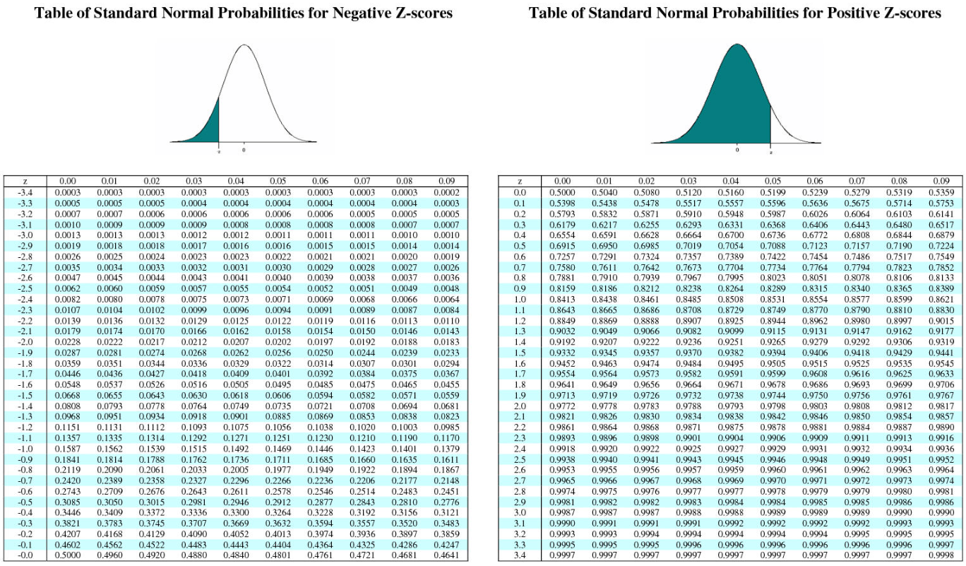
Computing Areas Under the Normal and t Distributions: To use the normal and $t$ distributions, we need to be able to calculate areas under the associated curves. In your introductory statistics class, you probably used a table that looks like this:

or this:

We will not use tables in this class, and instead will get the probabilities using R. We can use the following functions to compute these areas:

For the standard normal distribution (Z-distribution):
- pnorm(q): Computes the area to the left of the value q under the standard normal curve. If you want the area to the right of the value q, you can also get that using pnorm(q, lower.tail = FALSE).
- qnorm(p): Computes the value q such that the area to the left of q under the standard normal curve is equal to p. If you want the value of q such that the area to the right of q is p, you can also get that using qnorm(p, lower.tail = FALSE).
For the t-distribution with df degrees of freedom:
- pt(q, df): Computes the area to the left of the value q under the $t$-distribution curve with df degrees of freedom. It also has a lower.tail argument that you can use to use the right tail.
- qt(p, df): Computes the value q such that the area to the left of q under the t-distribution curve with df degrees of freedom is equal to p. It also has a lower.tail argument that you can use to use the right tail.

So, in the figure we got above for $T$-statistic on for the IQs in the wages dataset, if the mean were really 100 then:

The probability of seeing a $T$-statistic below 2.6 is pt(2.6, 934), which is 0.9952652.
The probability of seeing a $T$-statistic above 2.6 is pt(2.6, 934, lower.tail = FALSE), which is 0.0047348.
The value of $T$ such that we get below that statistic 75% of the time is qt(.75, 934), which is 0.6747525.
The value of $T$ such that we get above that statistic 75% of the time is qt(.75, 934, lower.tail = FALSE), which is -0.6747525.

5.5 Hypothesis Testing

Hypothesis testing is used to test a specific claim about the population. For example, in our treatment of IQ, we are interested in the specific claim that the average IQ in the population that we sampled from is equal to 100.

This involves formulating two competing hypotheses: the null hypothesis (often denoted as $H_0$) and the alternative hypothesis (denoted as $H_1$ or $H_a$). For the wages data, it makes sense to consider the following two hypotheses:

$H_0$: the population average IQ is 100 ($\mu = 100$).
$H_1$: the population average IQ is not 100 $(\mu \ne 100)$.

The goal of a hypothesis test is typically to disprove the null hypothesis. To do this, we engage in the following thought process:

Suppose that the null hypothesis were true, i.e., the average IQ really was 100. If that were the case, how unlikely would it be to observe the sample mean $\bar Y = 101.28$ that we actually observed, or something at least as extreme as this?

We proceed by calculating the $T$-statistic

\[ T = \frac{\bar Y - 100}{s_{\bar Y} / \sqrt N}. \]

Now, if we assume that the null hypothesis is true, then $\mu = 100$ is the population mean. Therefore if we assume that the null hypothesis is true then $T$ should have a $t$-distribution with $N - 1$ degrees of freedom.

OK, let’s compute the $T$-statistic for the IQ data now:

t_statistic <- (mean(wages$IQ) - 100) / (sd(wages$IQ) / sqrt(935))
print(t_statistic)

[1] 2.604958

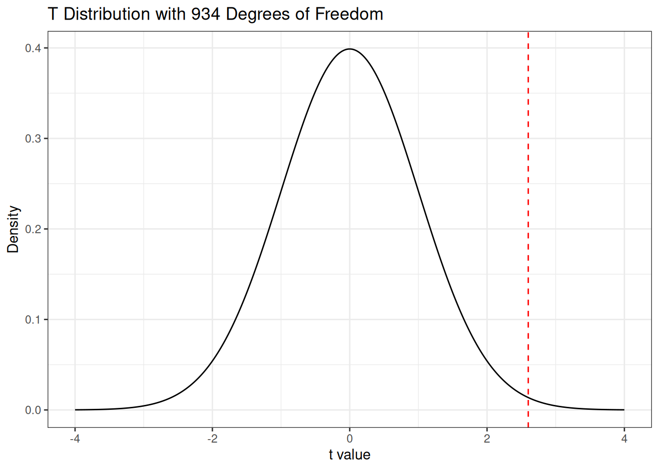
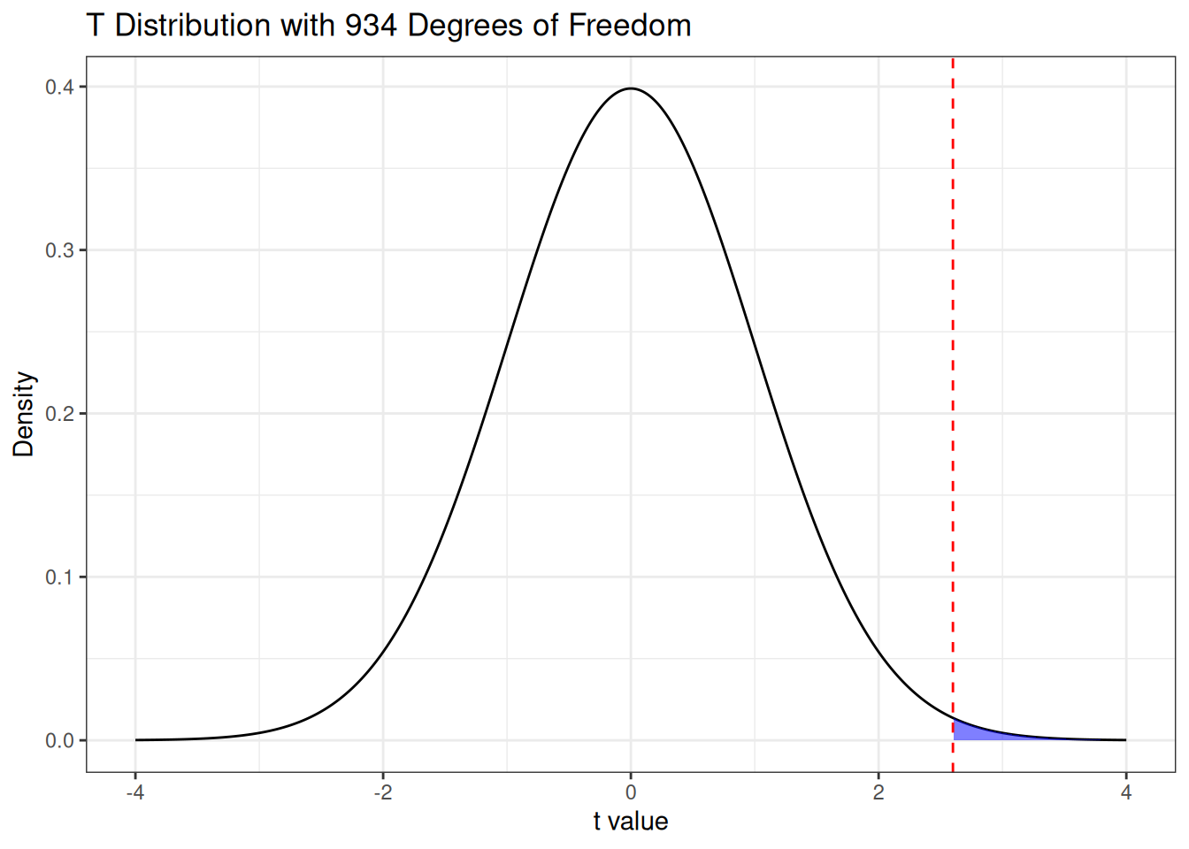
So, we have observed $T = 2.60$. We now ask: if the null hypothesis were true, would this be unusual? We can find out by referencing the $t$-distribution curve with $934$ degrees of freedom:

It looks like the value of $T$ we observed would be a bit unusual if the null hypothesis were true! How unusual? Well, we can identify all values of $T$ that are at least as extreme as what we observed as all of those either above $2.60$ or below $-2.60$, so we are interested in the probabilities under the curve illustrated below:

The “probability of observing a result at least as extreme as the one we observed, assuming the null hypothesis is true” is called a $P$-value. In this case, the $P$-value is given by

pt(2.6, 934, lower.tail = FALSE) + ## Probability above 2.6
  pt(-2.6, 934)                    ## Probability below -2.6

[1] 0.009469564

Roughly speaking, if the null hypothesis were true, we would get this result only one time in a hundred.

P-Value Cutoffs

By convention, many fields of science take a $P$-value of 0.05 (or smaller) as small enough that we can reject the null hypothesis. So, in many fields of science, observing the $P$-value of 0.009 would be sufficient to conclude that the population sampled from the wages data has an average IQ higher than 100.

If you work in the social, medical, or biological of sciences, you may have the impression that the $0.05$ cutoff is universal. In the “hard” sciences, however, the guidelines are actually quite a bit stricter. In physics, for example, the standard cutoff for a significant result is a “five sigma” result, which translates to a $P$-value less than 0.0000006. This is the benefit of working in a field that actually makes strong theoretical predictions with empirical backing, which the soft sciences usually do not.

My personal opinion is that the 0.05 cutoff is too high, and that science would be better served by more stringent cutoffs, as it seems like a lot of time is wasted in social sciences chasing small effects with dubious support. But, again, this is just my opinion. In their defense, part of the reason social scientists settle for these low cutoffs is that running studies is very expensive and there is usually not very strong economic incentives to run better studies.

In this course, we will treat the $P$-value as a measure of evidence against the null hypothesis; the smaller the $P$-value, the more evidence we have against the null. I’ll use the following informal guidelines for the cutoffs:

If the $P$-value is greater than 0.05, I will say that there is no evidence contradicting the null hypothesis.
If the $P$-value is between $0.01$ and $0.05$, I will say that there is weak evidence against the null hypothesis.
If the $P$-value is between $0.001$ and $0.01$, I will say that there is moderate evidence against the null hypothesis.
If the $P$-value is lower than $0.001$, I will say that there is strong evidence against the null hypothesis.

These are just guidelines in terms of how I will use the language, but depending on the context even a $P$-value less than 0.001 might not be very strong evidence against the null hypothesis.

5.5.1 The Role of the Alternative Hypothesis

In computing the $P$-value, it looks like we did not actually use the alternative hypothesis for anything! The role of the alternative hypothesis is actually that it determines what constitutes a “more extreme” outcome than what was observed. Suppose, for example, that we instead had the following null and alternative hypotheses:

$H_0$: $\mu = 100$.
$H_1$: $\mu < 100$.

This pair of hypothesis states that the IQ in the sampling population is equal than 100 (as the null) or less than 100 (as the alternative). In this scenario, if our sample mean is above $100$, it supports the null hypothesis rather than the alternative.

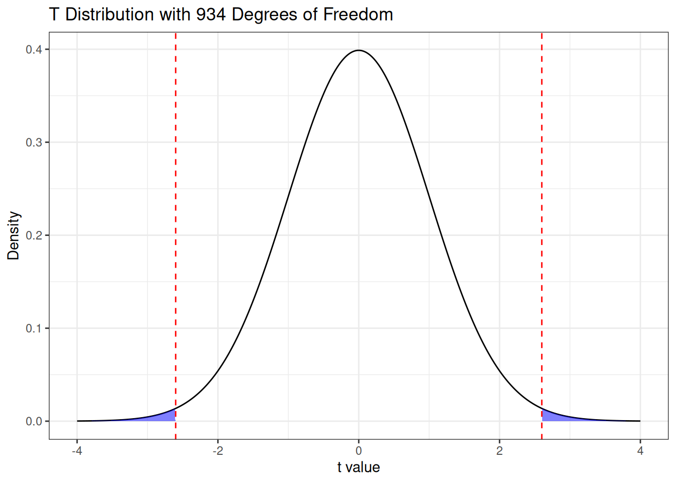
Under this alternative, the values of $\bar X$ that are “more extreme” (in the sense of providing more evidence in favor of the alternative) than the one we observed are all of the values of $\bar X$ smaller than the one we observed. Consequently, the $P$-value would be given by the area highlighted below:

This is given by

pt(2.6, df = 934)

[1] 0.9952652

So the $P$-value is close to $1$! We can conclude that there is basically no evidence in the data supporting the conclusion that the average IQ in the sampling population is less than 100.

On the other hand, consider the opposite hypotheses:

$H_0$: $\mu = 100$.
$H_1$: $\mu > 100$.

Then the values more extreme than the one we observed (in the sense of providing more evidence for the alternative) are the values of $\bar X$ larger than 100. So, we get a $P$-value associated with the highlighted region below:

So the $P$-value is

pt(2.6, df = 934, lower.tail = FALSE)

[1] 0.004734782

which is about 0.0047; the data provides moderate evidence against the null hypothesis that $\mu = 100$ in this case.

5.6 Confidence Intervals

Rather than performing a test, let’s say that I just want a plausible range of values for the average IQ in the sampling population. To do this, we can build a confidence interval. Confidence intervals are used to find, for some population quantity, an interval of plausible values for that quantity. Confidence intervals are set up to have the following property:

Coverage of a Confidence Interval

A (random) interval with lower endpoint $L$ and upper endpoint $U$ is said to be a $100(1 - \alpha)\%$ confidence interval for a population quantity $\beta$ if

\[ \Pr(L \le \beta \le U) = 1 - \alpha. \]

That is, if we replicated our data collection procedure infinitely many times, then we would find that $\beta$ is not between $L$ and $U$ in $100 \alpha\%$ of the replications, i.e., the interval makes a mistake with probability $\alpha$.

As a concrete example, let’s suppose that the population average IQ really is 100. If we make a 95% confidence interval for the population average IQ for the wages dataset, what this means is that, if we collected many different wages datasets from the population, then on 5% of these datasets the interval we make will fail to include the value 100.

Important

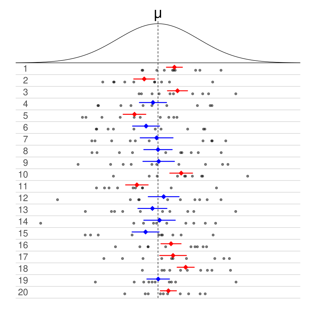
In the above definition, the quantity $\beta$ is not random. The randomness of the confidence interval comes from the fact that different replications of the data collection lead to different confidence intervals. A picture of this is given below:

Twenty samples of normally distributed data are shown in rows. Directly above each sample is the 50% confidence interval for the mean, with the sample mean marked with a diamond. Intervals that include the mean are blue, and the rest are red.Borrowed with permission under the Creative Commons license from https://commons.wikimedia.org/wiki/File:Normal_distribution_50%25_CI_illustration.svg.

The figure consists of 20 repeated samples of data from a normal distribution with some mean $\mu$; for each sample of points, a 50% confidence interval is created. The mean of the distribution does not change across the samples! Instead, we see that about 50% of the intervals that get made contain the true mean (blue) while about 50% do not (red).

We now show how to get a confidence interval for the population average $\mu$. Starting from the $T$-statistic, note that if we compute

\[ T = \frac{\bar X - \mu}{s / \sqrt N} \]

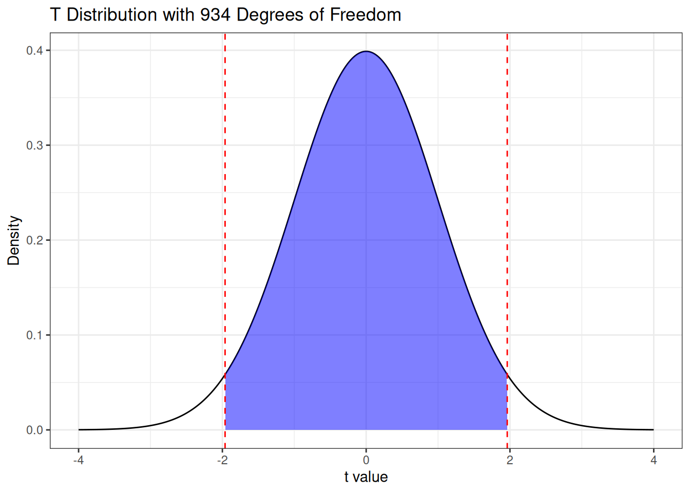
then we would expect (with 95% probability) $T$ to be between the highlighted regions below:

We expect it to be between the vertical bars because these have been chosen to make the shaded area equal to 95%. So we have

\[ -1.96 \le \frac{\bar X - \mu}{s / \sqrt N} \le 1.96 \qquad \text{with probability 95\%}. \]

To express this inequality in terms of $\mu$, we rearrange the terms as follows:

\[ -1.96 \le \frac{\bar{X} - \mu}{s / \sqrt{N}} \le 1.96 \]

Multiplying all parts by $\frac{s}{\sqrt{N}}$, we obtain:

\[ -1.96 \times \frac{s}{\sqrt{N}} \le \bar{X} - \mu \le 1.96 \times \frac{s}{\sqrt{N}} \]

Finally, adding $\mu$ to all parts, we get:

\[ \bar{X} - 1.96 \times \frac{s}{\sqrt{N}} \le \mu \le \bar{X} + 1.96 \times \frac{s}{\sqrt{N}} \]

More generally, if we have a desired confidence level $1 - \alpha$ (so that the confidence interval will fail to catch the true value of $\mu$ with probability $100\alpha\%$), then the confidence interval we get is

\[ \bar X - t_{\alpha/2} \times \frac{s}{\sqrt N} \le \mu \le \bar X + t_{\alpha/2} \times \frac{s}{\sqrt N} \]

where $t_{\alpha/2}$ is the the $100(1 - \alpha/2)$’th percentile of the $t$-distribution with $N - 1$ degrees of freedom.

Applying the above formula, a confidence interval for the average IQ test score in the population is

avg_iq <- mean(wages$IQ)
sd_iq <- sd(wages$IQ)
alpha <- 0.05
t <- qt(p = 1 - alpha / 2, df = 934, lower.tail = TRUE)
lower_limit <- avg_iq - t * sd_iq / sqrt(935)
upper_limit <- avg_iq + t * sd_iq / sqrt(935)
print(c(lower_limit = lower_limit, upper_limit = upper_limit))

lower_limit upper_limit 
   100.3163    102.2484

Hence, our 95% confidence interval for the average IQ in the sample is that it is between 100.31 and 102.24.

5.7 Hypothesis Tests and Confidence Intervals Using R for a Mean

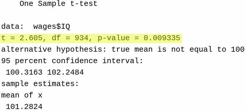
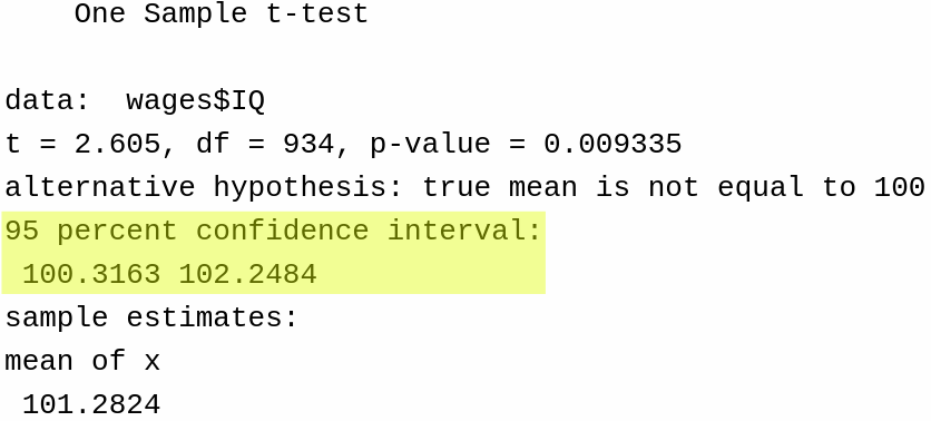
To apply a hypothesis test of the null $H_0: \mu = 100$ against the alternative $H_a: \mu \ne 100$, we can run the following code:

t.test(wages$IQ, mu = 100)


    One Sample t-test

data:  wages$IQ
t = 2.605, df = 934, p-value = 0.009335
alternative hypothesis: true mean is not equal to 100
95 percent confidence interval:
 100.3163 102.2484
sample estimates:
mean of x 
 101.2824

The main results of the test are given here:

We can also change the alternative hypothesis to be $\mu > 100$ by running this code:

t.test(wages$IQ, alternative = 'greater', mu = 100)


    One Sample t-test

data:  wages$IQ
t = 2.605, df = 934, p-value = 0.004667
alternative hypothesis: true mean is greater than 100
95 percent confidence interval:
 100.4718      Inf
sample estimates:
mean of x 
 101.2824

or we can set $H_a: \mu < 100$ by running this code:

t.test(wages$IQ, alternative = "less", mu = 100)


    One Sample t-test

data:  wages$IQ
t = 2.605, df = 934, p-value = 0.9953
alternative hypothesis: true mean is less than 100
95 percent confidence interval:
     -Inf 102.0929
sample estimates:
mean of x 
 101.2824

The output of the t.test() also includes a confidence interval, which is given here:

5.8 Statistical Versus Practical Significance

When interpreting the results of an analysis it is important to bear in mind that statistical significance is not the same as practical significance. To make the point, our 95% confidence interval for the sampling population IQ was

\[ 100.31 \le \text{avg. IQ} \le 102.24. \]

While this is a statistically significant difference, it does not (to me) seem practically significant. Practical significance addresses the question: “Is this difference important or valuable in practice?” Even at the high end, the difference in IQ is only 2 points from the hypothesized average IQ of 100. Determining whether a difference is practically significant depends on the context of the problem you are trying to solve. It’s hard to say in this case because we did not have a specific problem to solve when introducing this dataset. However, for most purposes, I would not view a difference of 1-2 IQ points as practically meaningful.

Another example: The problem of practical significance often arises in clinical settings. For example, we might consider a large-scale clinical trial for a new blood pressure medication. Let’s say the study involves 10,000 patients with hypertension, comparing the new drug to the standard of care. After a 6-month treatment period, the results show:

Mean systolic blood pressure reduction in the treatment group: 12 mmHg
Mean systolic blood pressure reduction in the standard of care group: 11 mmHg
The difference is statistically significant with a p-value < 0.001

In this case, we have strong statistical evidence that the new medication outperforms the standard of care medication. However, when we look at the actual effect size – a mere 1 mmHg difference in blood pressure reduction – we need to consider whether this is practically significant. Most clinicians would not consider a 1 mmHg difference in blood pressure meaningful for an individual patient’s health outcomes; on the other hand, the new drug might be more expensive, or have more side effects, and so the minimal benefit might not justify these potential drawbacks.

5.9 Exercises

5.9.1 Exercise: The Sampling Population

You are tasked with studying the effectiveness of a new online learning platform for high school students.

Identify a suitable target population for this study.
Describe how you might go about designing a study that (tries to) sample from this population. How would you select participants for your study?.
Discuss at least two ways in which your sampling population might differ from the target population. How might these differences impact the conclusions you can draw from your study?
Explain the difference between the “population” average effect of using the new learning platform and the “sample” average effect, where the effect of the learning platform is defined as the difference between the score of a student on a test after trying the learning platform and their score on a pre-test.

5.9.2 Exercise: Random Variables

Consider the following experiment: A researcher is studying the effect of a new fertilizer on tomato plants. They randomly assign 50 tomato plants to receive either the new fertilizer or a standard fertilizer. After 30 days, they take measurements on each plant.

For each of the following measurements, determine whether it could be considered a random variable. If it is a random variable, briefly explain why. If it is not a random variable, explain why not and suggest how it could be transformed into a random variable.

The height of the plant in centimeters.
Whether the plant survived (yes or no).
The color of the tomatoes produced (red, orange, or yellow).
The number of tomatoes produced by each plant.
The overall health of the plant (poor, fair, good, excellent).
The weight of all tomatoes produced by a plant in grams.

5.9.3 Exercise: Some Simple Probability

Consider a deck of 52 cards numbered 1 (Ace) through 13 (King) with four suits (hearts, diamonds, clubs, and spades). You draw one card randomly from this deck. Let $X$ be the random variable representing the number on the drawn card.

List all possible outcomes and their probabilities.
Calculate the probability of drawing a card with a number greater than 7.
Calculate the expected value (mean) of $X$.
Calculate the variance of $X$. Show your work for each part.
Let $Y$ be equal to $0$ if we draw a heart or diamond, and equal to the value of the card if we draw a spade or club. What is the PMF associated to $Y$?
Compute the expected value and standard deviation of $Y$.

5.9.4 Exercise: More Probability

Suppose that we roll a fair six-sided die. What are the probability mass functions of the following random variables:

$X = 1$ if the outcome is divisible by 3 and $X = 0$ otherwise.
$X =$ the number on face-up side of the die.
$X =$ the square of the number on the face-up side of the die.

5.9.5 Exercise: Discrete or Continuous?

Classify each of the following random variables as either discrete or continuous. If you’re unsure about any, explain your thinking – there might be room for debate!

The number of times you hit snooze on your alarm before finally getting up for class.
The amount of caffeine (in milligrams) in your third cup of coffee today.
The number of unanswered emails in your inbox right now.
The battery percentage on your phone.
Your GPA at the end of this semester.
The distance between you and the nearest pizza place.
The volume level on your headphones.
The time it takes to find a parking spot on campus.

5.9.6 Exercise: The Normal Distribution

Assume that IQ scores follow a normal distribution with a mean of 100 and a standard deviation of 15. Use the R functions pnorm and qnorm to answer the following questions:

What is the probability that a randomly selected individual has an IQ less than 85.
What is the probability that a randomly selected individual has an IQ greater than 115.
What is the probability that a randomly selected individual has an IQ between 90 and 110.
Suppose that someone has an IQ that is higher than 98% of the population. What is this individual’s IQ?
Using the probabilities computed above, explain how these relate to the definition of a probability in terms of relative frequencies.
Explain why the answers to part (a) and part (b) are the same.
Without using any R function, what percentage of the population has an IQ between 55 and 145?

5.9.7 Exercise: Looking at the Wage Variable

Load the wages dataset by running the following code:

filename <- "https://raw.githubusercontent.com/theodds/SDS-348/master/wages.csv"
wages <- read.csv(filename) %>% select(-X)

What is your estimate of the average monthly wage of an individual in the population?
What is the standard error (i.e., precision) of this estimate?
Is this estimator biased?
Make a 95% confidence interval for the average monthly wage of individuals in the population.
Make a 99.999% confidence interval for the average monthly wage of individuals in the population.
Test the null hypothesis that the average monthly wage is equal to $900 against the alternative that it is greater than $900. What is the $P$-value of this test? How strong is the evidence against this null?
What is the $T$-statistic for the test in part f? Compute it without using the t.test function.

5.9.8 Exercise: Central Limit Theorem

Explain the Central Limit Theorem in your own words.
Given a population with a mean of 50 and a variance of 25, explain how the distribution of the sample mean $\bar X$ changes as the sample size $N$ increases. Use sample sizes of 5, 30, and 100 for your explanation.
Calculate the standard error of the sample mean for each of the sample sizes mentioned.

5.9.9 Exercise: More Hypothesis Testing

Imagine you own an ice cream shop and believe the average number of ice cream cones sold per day is 120. You sample 16 days and find an average of 125 ice creams sold per day with a sample standard deviation of 10.

Formulate the null hypothesis $H_0$ and the alternative hypothesis $H_1$.
Calculate the T-statistic for your sample mean.
Find the critical T-value for a 0.05 significance level with the appropriate degrees of freedom.
Determine whether to reject the null hypothesis.

5.9.10 Exercise: More Confidence Intervals

Suppose you surveyed 30 people about their rating of a new movie, and the average rating is 8.2 on a 0 to 10 scale with a sample standard deviation of 1.5.

Calculate the 95% confidence interval for the true mean rating of the movie.
Interpret the confidence interval in the context of the movie’s rating.
What percentage of individuals rated the movie more than 2 standard deviations above the average?

5.9.11 Exercise: Distinguishing Statistical and Practical Significance

A company conducts a study to determine whether a new training program significantly improves employee productivity. The study finds a statistically significant increase in productivity (p-value < 0.01), but the actual improvement is only 0.5% more tasks completed per day compared to the old training program.

What factors should the company consider to determine if the 0.5% increase in productivity is practically significant?
How might the cost of the new training program, employee satisfaction, and long-term benefits influence the decision to implement the new program?
Can you think of a situation where a small, statistically significant difference would be practically significant? Provide an example and justify your reasoning.

Wooldridge Source: M. Blackburn and D. Neumark (1992), “Unobserved Ability, Efficiency Wages, and Interindustry Wage Differentials,” Quarterly Journal of Economics 107, 1421-1436↩︎
http://compcogscisydney.org/learning-statistics-with-r ↩︎
A more formal definition of discrete random variables is that they can take on a countable number of possible outcomes.↩︎
A more formal definition of continuous random variables is that $X$ is continuous if the function $F(x) = \Pr(X \le x)$ is a continuous function.↩︎
https://www.johndcook.com/blog/2008/07/20/why-heights-are-not-normally-distributed/↩︎