In this chapter we look at another alternative to linear regression. This time, rather than looking at success/failure data, we will instead look at data that can be represented as counts, such as the number of occurrences of an event.
16.1 Motivating Example: Epilepsy Data
In this chapter, we examine data from the MASS package to investigate the effect of the drug progabide on the number of seizures experienced by epileptic patients over a two-week period. According to the dataset’s documentation:
Thall and Vail (1990) give a data set on two-week seizure counts for 59 epileptics. The number of seizures was recorded for a baseline period of 8 weeks, and then patients were randomly assigned to a treatment group or a control group. Counts were then recorded for four successive two-week periods. The subject’s age is the only covariate.
We can load the data as follows:
library(tidyverse)epil <- MASS::epilepil <-subset(epil, period ==4, select =-c(period, V4))head(epil)
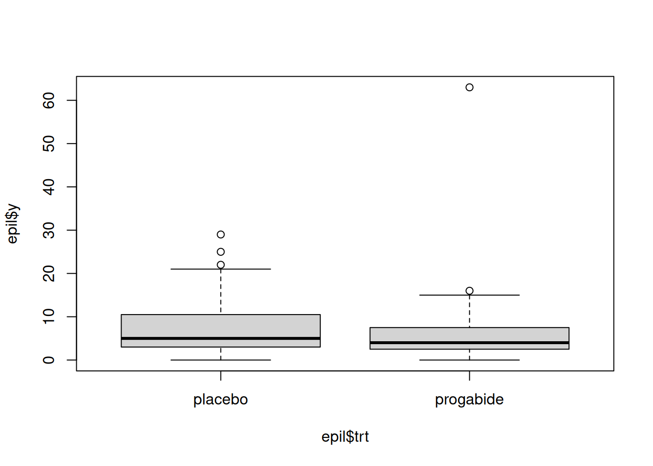
The main variable of interest is y, which represents the number of seizures recorded during the final two-week period of the study. The variable trt indicates whether the patient received the placebo or progabide treatment. To explore the relationship between these variables, we can use a boxplot:
boxplot(epil$y ~ epil$trt)
From the boxplot, it appears that individuals in the treatment group tend to have lower seizure counts. However, the presence of an extreme outlier in the treatment group complicates this interpretation. If we were to naively perform a two-sample t.test to compare the groups, we would find no significant evidence of a difference:
t.test(epil$y ~ epil$trt)
    Welch Two Sample t-test

data:  epil$y by epil$trt
t = 0.50505, df = 53.012, p-value = 0.6156
alternative hypothesis: true difference in means between group placebo and group progabide is not equal to 0
95 percent confidence interval:
 -3.727891  6.237108
sample estimates:
  mean in group placebo mean in group progabide
               7.964286                6.709677
Evidently, if we stopped here, we would not be able to conclude that progabide does anything. To better understand the treatment’s impact, we should also consider additional variables:
age: The age of the subject, as the treatment’s effectiveness may vary across age groups.
base: The number of seizures the patient experienced during a two-week period before treatment. This variable is crucial for determining whether the treatment reduces seizure counts, as it helps account for baseline severity of epilepsy. Patients who have severe epilepsy symptoms will typically have more seizures even after treatment, and accounting for this can be important in determining whether the treatment is effective.
Our goal: The question we are interested in is whether progabide reduces the number of seizures that patients experience on average and, if so, by how much.
16.2 Why Do We Need Poisson Regression
Similar to logistic regression, we might hope that multiple linear regression is already up to the task of modeling a count outcome \(Y_i\). However, when \(Y_i\) is a count, most of the assumptions of linear regression are usually violated:
For count data, the relationship between \(Y_i\) and \(X_{ij}\) is usually not linear. For instance, plugging in very large or small values for \(X_{ij}\) can lead to nonsensical predictions, such as negative values for \(Y_i\). Thus, the linearity assumption is typically violated.
Counts often exhibit greater variability for higher predicted values. For example, in Austin, we might predict close to zero earthquakes annually with high confidence. In contrast, for Los Angeles, we might (i) predict more earthquakes and (ii) anticipate greater uncertainty in our prediction. This violates the constant variance assumption, as variability depends on the magnitude of the predicted count.
Because counts can only take on specific values \(0, 1, 2, \ldots\) we know immediately that \(Y_i\) cannot have a normal distribution. So the normality assumption of the errors is violated.
Optional: Some People Still Use Linear Models for Counts
Unlike with success/failure data, linear regression is occasionally used for count outcomes. The main concern is the violation of the constant variance assumption, which can sometimes be addressed by transforming the outcome using \(\sqrt{Y_i}\). The main downside of this approach is that we usually want to predict \(Y_i\) directly rather than \(\sqrt Y_i\).
16.3 The Poisson Distribution
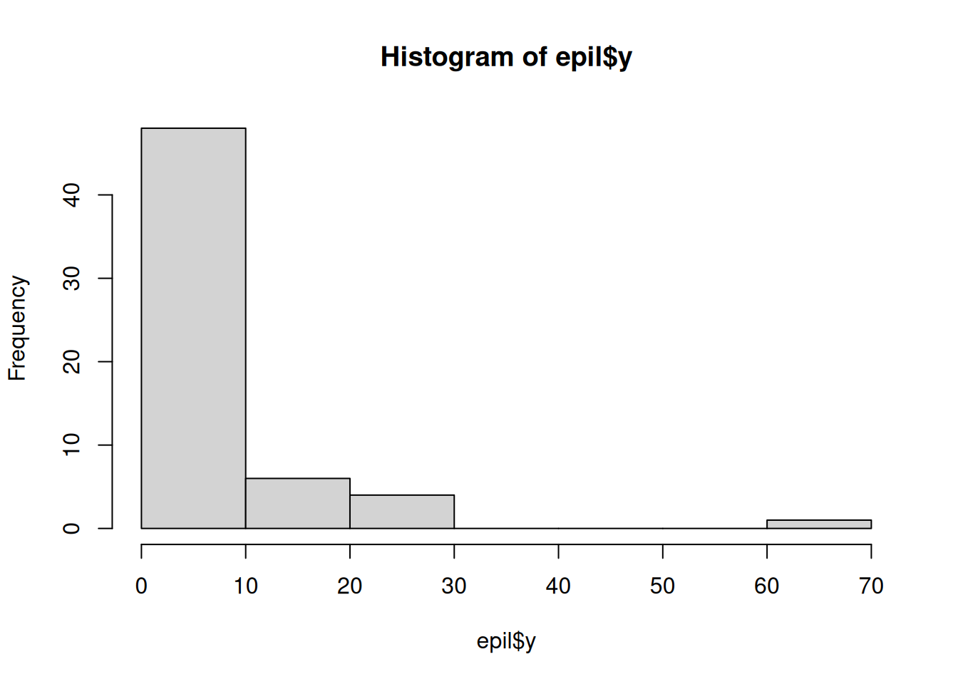
By their nature, count data do not follow a normal distribution: they are non-negative, take only whole number values, and are often skewed. For example, this skewness is evident in the epilepsy dataset:
hist(epil$y)
The simplest and most commonly used distribution for modeling count data is the Poisson distribution.
Definition: The Poisson Distribution
A random variable \(Y\) is said to have a Poisson distribution with mean \(\mu\) if
\[
\Pr(Y = y) = \frac{\mu^y e^{-\mu}}{y!}
\]
for \(y = 0, 1, 2, \cdots\).
The Poisson distribution has two key characteristics:
The mean \(\mu\) equals the variance, i.e., \(\text{Var}(Y) = \mu\).
It is skewed when \(\mu\) is small but becomes more symmetric as \(\mu\) increases, making it well-suited for data with smaller counts.
Optional: Why the Poisson Distribution in Particular?
The reason that the Poisson distribution is popular for count data is that it arises mathematically as a model for the number of events occurring in a fixed interval of time, given that these events happen independently and with a constant rate of occurrence over time. For more details, see here.
Quantities often modeled using the Poisson distribution include:
The number of car accidents at an intersection in a year.
The number of people in line at a specific time.
The number of photons hitting a detector in a given period.
The number of earthquakes in a city over a given time.
The number of seizures experienced by an individual in a given period.
16.4 The Poisson Log-Linear Model
For count data, the starting point is the Poisson log-linear model, which relates the mean \(\mu_i\) of the outcome \(Y_i\) to the independent variables using the following equation:
This model ensures that \(\mu_i\), the mean of \(Y_i\), remains positive, as the exponential function \(e^x\) is always positive. This is important because \(Y_i\) is always non-negative, so its average should also be non-negative.
The Poisson log-linear model makes the following assumptions:
Linearity: the quantity \(\ln \mu_i\) is linearly related to the independent variables, \(\ln \mu_i = \beta_0 + \sum_{j = 1}^P \beta_j \, X_{ij}\).
Independence: The outcomes \(Y_i\) are independent of each other. For example, in the epilepsy dataset, the number of seizures experienced by one patient should not affect the number of seizures experienced by another.
Poisson Outcomes: The outcomes \(Y_i\) follow a Poisson distribution with mean \(\mu_i\).
Each of these assumptions is important for the statistical inferences we get from a Poisson log-linear model to be valid. Of these assumptions, the weak point is often that the \(Y_i\)’s truly follow a Poisson distribution. Later in this chapter, we discuss one approach to address violations of this assumption.
16.4.1 Fitting the Poisson Log-Linear Model
Like logistic regression, the coefficients of the Poisson log-linear model are estimated using maximum likelihood estimation (MLE). Specifically, the coefficients are chosen to maximize the likelihood function:
16.5 Interpreting the Coefficients of the Poisson Log-Linear Model
The coefficients of the Poisson log-linear model have an interpretation similar to those in log-transformed linear regression, which we saw in Chapter 11. Specifically:
Interpretation of the Coefficients of a Poisson Log-Linear Model
Holding all other independent variables constant, increasing \(X_{ij}\) by one unit leads to multiplying the mean by \(e^{\beta_j}\). For example, if \(\beta_j
= 2\) then increasing \(X_{ij}\) by one unit results in multiplying the mean of \(Y_i\) by \(e^2 = 7.389\).
16.5.1 Derivation of the Interpretation
To see why this is true, suppose that observations \(i = 1\) and \(i = 2\) are identical except for the fact that \(X_{2j}\) is one unit larger than \(X_{1j}\). Then we can write:
This shows that \(\mu_2\) is \(\mu_1\) multiplied by \(e^{\beta_j}\), confirming the interpretation that a one-unit increase in \(X_{ij}\) leads to multiplying the mean by \(e^{\beta_j}\).
16.6 Fitting Log-Linear Models with glm
Similar to logistic regression, the Poisson log-linear model is fit in R using the glm function. To fit a Poisson log-linear model, we simply set the family argument to poisson instead of binomial.
16.6.1 Example: The Epilepsy Dataset
For the epilepsy dataset, we model y (the number of seizures) as the dependent variable and use age, trt, and base as independent variables:
epil_poisson <-glm(y ~ age + trt + base, data = epil, family = poisson)
We can then use summary() to view the results of the analysis:
summary(epil_poisson)
Call:
glm(formula = y ~ age + trt + base, family = poisson, data = epil)

Coefficients:
              Estimate Std. Error z value Pr(>|z|)
(Intercept)   0.775574   0.284598   2.725  0.00643 **
age           0.014044   0.008580   1.637  0.10169
trtprogabide -0.270482   0.101868  -2.655  0.00793 **
base          0.022057   0.001088  20.267  < 2e-16 ***
---
Signif. codes:  0 '***' 0.001 '**' 0.01 '*' 0.05 '.' 0.1 ' ' 1

(Dispersion parameter for poisson family taken to be 1)

    Null deviance: 476.25  on 58  degrees of freedom
Residual deviance: 147.02  on 55  degrees of freedom
AIC: 342.79

Number of Fisher Scoring iterations: 5
Interpreting the coefficients of this output, we have:
Age: For every additional year of age, the mean number of seizures increases by a factor of \(e^{0.014044} \approx 1.014\). This corresponds to a 1.4% increase in the number of seizures for each additional year.
Treatment (trt): Individuals treated with progabide have their mean number of seizures multiplied by \(e^{-0.270482} \approx 0.763\). This means treated individuals are estimated to experience, on average, roughly 76% as many seizures as they would without treatment.
Baseline seizures (base): Each additional seizure during the baseline period increases the estimated mean number of seizures by a factor of \(e^{0.022057} \approx 1.022\), equivalent to a 2.2% increase per baseline seizure.
16.7 Getting the Predictions from the Model
We can generate predictions from the model using the predict() function, as in logistic regression. For example, suppose we want predictions for an individual with the following attributes:
Age: 30 years.
Baseline seizures: 10.
Predictions for both placebo and progabide treatment.
First, we create a new data frame to represent these scenarios:
Then, we use the predict() function to obtain the predictions:
predict(epil_poisson, new_data, type ="response")
       1        2
4.126611 3.148651
In this case, the model predicts approximately 4 seizures for the placebo group and 3 seizures for the treated group.
Make Sure to Set type = response
As with logistic regression, you must set type = "response" in the predict() function to obtain the estimated mean (\(\mu_i\)). If you omit this, the function returns predictions for \(\ln \mu_i\) instead. For example:
predict(epil_poisson, new_data)
       1        2
1.417456 1.146974
This output is the natural logarithm of the estimated mean. To confirm, you can take the logarithm of the predicted means:
log(predict(epil_poisson, new_data, type ='response'))
       1        2
1.417456 1.146974
If you omit the new_data argument, the predict() function will provide predictions for the original dataset:
16.8 Statistical Inference With Poisson Log-Linear Models
Another similarity between Poisson log-linear models and logistic regression models is that we should generally do statistical inference using the anova() and drop1() functions (for testing) rather than relying on the output of summary(), as the \(P\)-values in the output of summary() are not very reliable. Using drop1()we can get the \(P\)-values for the significance of the independent variables (assuming that the other independent variables are controlled for):
drop1(epil_poisson, test ="LRT")
Single term deletions

Model:
y ~ age + trt + base
       Df Deviance    AIC    LRT  Pr(>Chi)
<none>      147.02 342.79
age     1   149.68 343.44   2.65  0.103244
trt     1   154.10 347.87   7.08  0.007788 **
base    1   467.77 661.54 320.75 < 2.2e-16 ***
---
Signif. codes:  0 '***' 0.001 '**' 0.01 '*' 0.05 '.' 0.1 ' ' 1
The results from drop1() may differ from those in summary(). When discrepancies arise, the output of drop1() should be preferred. The drop1() function performs single-term deletion tests, which test hypotheses like the following for the age variable:
\(H_0\): Age does not impact the average number of seizures, controlling for trt and base (\(\beta_{\texttt{age}} = 0\)).
\(H_1\):Age does impact the average number of seizures, controlling for trt and base (\(\beta_{\texttt{age}} \neq 0\))).
In contrast, anova() performs sequential tests, where variables are added to the model one at a time:
anova(epil_poisson, test ="LRT")
Analysis of Deviance Table

Model: poisson, link: log

Response: y

Terms added sequentially (first to last)

     Df Deviance Resid. Df Resid. Dev Pr(>Chi)
NULL                    58     476.25
age   1     4.42        57     471.83  0.03561 *
trt   1     4.06        56     467.77  0.04382 *
base  1   320.75        55     147.02  < 2e-16 ***
---
Signif. codes:  0 '***' 0.001 '**' 0.01 '*' 0.05 '.' 0.1 ' ' 1
Now, the row for age tests the following hypotheses:
\(H_0\): Age does not improve predictions compared to a model with only an intercept.
\(H_1\): Age improves predictions compared to a model with only an intercept.
The conclusions are somewhat different, as it appears there is evidence that age is useful on its own but is less useful if we are already accounting for base and trt.
16.8.1 Testing for Overall Model Significance
To test the overall significance of the model, we compare the full model to an intercept-only model:
epil_intercept_only <-glm(y ~1, data = epil, family = poisson)anova(epil_intercept_only, epil_poisson, test ="LRT")
Analysis of Deviance Table

Model 1: y ~ 1
Model 2: y ~ age + trt + base
  Resid. Df Resid. Dev Df Deviance  Pr(>Chi)
1        58     476.25
2        55     147.02  3   329.23 < 2.2e-16 ***
---
Signif. codes:  0 '***' 0.001 '**' 0.01 '*' 0.05 '.' 0.1 ' ' 1
A small \(P\)-value indicates that we reject the null hypothesis (\(H_0\)) that all coefficients are zero, and conclude that at least one of age, trt, or base contributes to predicting y.
16.8.2 Confidence Intervals
Confidence intervals for the coefficients can be obtained using the confint() function:
confint(epil_poisson)
                   2.5 %      97.5 %
(Intercept)   0.21310504  1.32915539
age          -0.00286682  0.03078313
trtprogabide -0.47078428 -0.07120030
base          0.01990601  0.02417532
For example, we might interpret the treatment effect as follows:
Holding age and baseline seizure count constant, we are 95% confident that individuals treated with progabide have between \(e^{-0.4708} \approx 0.625\) and \(e^{-0.0712} \approx 0.93\) times as many seizures as those given a placebo.
16.9 The Quasi-Poisson Model
The big drawback of the Poisson log-linear model is the assumption that the \(Y_i\)’s follow a Poisson distribution. This assumption is actually very restrictive! The main issue is that the Poisson distribution has only a single quantity - the mean \(\mu_i\) - that determines the entire shape of the distribution. Specifically, for Poisson random variables the mean also completely determines the spread:
\[
\text{Var}(Y_i) = \mu_i
\]
For comparison, the normal distribution has two parameters (\(\mu\) and \(\sigma^2\)) that separately control the mean and variance. In the Poisson model, the mean \(\mu_i\) does double duty, determining both the center and variability of \(Y_i\).
This limitation often makes the Poisson log-linear model unsuitable in practice. A more flexible alternative is the quasi-Poisson model, which introduces an additional parameter \(\phi\) to separately control the spread. The variance is modeled as:
\[
\text{Var}(Y_i) = \phi \, \mu_i
\]
The variance still depends on the mean, which is desirable for count data, but it is not completely determined by it.
To use the quasi-Poisson model, we change the family argument to quasipoisson:
epil_quasi <-glm(y ~ trt + age + base, data = epil, family = quasipoisson)summary(epil_quasi)
Call:
glm(formula = y ~ trt + age + base, family = quasipoisson, data = epil)

Coefficients:
              Estimate Std. Error t value Pr(>|t|)
(Intercept)   0.775574   0.448580   1.729   0.0894 .
trtprogabide -0.270482   0.160563  -1.685   0.0977 .
age           0.014044   0.013524   1.038   0.3036
base          0.022057   0.001715  12.858   <2e-16 ***
---
Signif. codes:  0 '***' 0.001 '**' 0.01 '*' 0.05 '.' 0.1 ' ' 1

(Dispersion parameter for quasipoisson family taken to be 2.484378)

    Null deviance: 476.25  on 58  degrees of freedom
Residual deviance: 147.02  on 55  degrees of freedom
AIC: NA

Number of Fisher Scoring iterations: 5
This model estimates \(\phi \approx 2.48\) (which is called the “Dispersion Parameter” in the output). Interestingly, there is no longer significant evidence that the treatment is effective. This result can be confirmed using drop1():
drop1(epil_quasi, test ="LRT")
Single term deletions

Model:
y ~ trt + age + base
       Df Deviance scaled dev. Pr(>Chi)
<none>      147.02
trt     1   154.10       2.850  0.09135 .
age     1   149.68       1.069  0.30127
base    1   467.77     129.106  < 2e-16 ***
---
Signif. codes:  0 '***' 0.001 '**' 0.01 '*' 0.05 '.' 0.1 ' ' 1
Unfortunately, this suggests that there is not much evidence that progabide reduces seizures.
Practical Advice: Use the Quasi-Poisson Model If Possible
Whenever possible, use the quasi-Poisson model instead of the Poisson log-linear model. The quasi-Poisson model is more flexible and avoids the pitfalls of assuming that variance equals the mean. However, note that a limitation of the quasi-Poisson model is that it does not provide prediction intervals.
There is little justification for using the Poisson log-linear model when the quasi-Poisson model is readily available. Using the Poisson model inappropriately can lead to misleading conclusions, as we saw on the epilepsy dataset.
16.10 Exercises
16.10.1 Exercise: Sprays
This exercise concerns data on a treatment for insects. The idea is that a different spray type was applied to different plants and, after some time, the number of insects on those plants was counted; more effective sprays should have fewer insects on them.
First, we load the data
data(InsectSprays)head(InsectSprays)
  count spray
1    10     A
2     7     A
3    20     A
4    14     A
5    14     A
6    12     A
The dataset has two columns:
count is the number of insects found on a plant after being treated with an insecticidal spray.
spray is the type of spray applied to the plan.
Noting that the outcome being measured (count) is a count variable, why might we want to avoid using a linear regression model for this data? Specifically, prior to fitting a linear model to this data, what assumption should we expect to be violated?
Having guessed at why linear regression may not end up working so well, go ahead and fit a linear regression using count as the outcome and spray as the predictor. Then, run the autoplot function on the output. Do the results of autoplot validate your guess? Explain.
Fit a Poisson loglinear model with count as the outcome and spray as the predictor. Then, test this model against a model including only the intercept using the anova function. Does there appear to be evidence that spray is related to the outcome?
Interpret the slopes estimated from the model in terms of a multiplicative effect on the number of insects relative to the baseline spray.
What is the estimated average number of insects for each of the sprays? Which spray does the best? Does this agree with the linear model?
16.10.2 Exercise: Crabs
The following crabs dataset contains data collected on female crabs. During spawning season, female crabs may attract a group of “satellite” male crabs that orbit around the female and try to fertilize her eggs. We load the data as follows:
# A tibble: 6 × 5
  color  spine width satell weight
  <chr>  <chr> <dbl>  <dbl>  <dbl>
1 medium bad    28.3      8   3050
2 dark   bad    22.5      0   1550
3 light  good   26        9   2300
4 dark   bad    24.8      0   2100
5 dark   bad    26        4   2600
6 medium bad    23.8      0   2100
Our goal is to understand what features of the female are associated with attracting many satellites. The variables are:
color: the color of the female crab (light, medium, dark, darker).
spine: the condition of the spine (bad, middle, good).
width: the width of the crab’s carapace in centimeters.
weight: the weight of the crab in grams.
satell: the number of satellites.
Fit a Poisson loglinear regression model, then interpret the slope associated to the weight of the female crabs in terms of the number of satellites she is expected to attract.
Is there evidence that the variable width is relevant for predicting the number of satellites, after controlling for the other variables? Test this using either anova or drop1, depending on which is appropriate for this question.
Is there evidence that width is relevant for predicting the number of satellites, if we do not include weight as a predictor? Test this using anova or drop1, depending on which is appropriate for answering this question.
What is the predicted number of satellites for (i) a light crab with a bad spine that is 28.3 centimeters wide and 3050 grams and (ii) a dark crab with a good spine, 25 centimeters wide and 2500 grams?
16.10.3 Exercise: DebTrivedi
The MixAll package contains the dataset DebTrivedi, which is described below:
Deb and Trivedi (1997) analyze data on 4406 individuals, aged 66 and over, who are covered by Medicare, a public insurance program. Originally obtained from the US National Medical Expenditure Survey (NMES) for 1987/88, the data are available from the data archive of the Journal of Applied Econometrics. It was prepared for an R package accompanying Kleiber and Zeileis (2008) and is also available as DebTrivedi.rda in the Journal of Statistical Software together with Zeileis (2006). The objective is to model the demand for medical care -as captured by the number of physician/non-physician office and hospital outpatient visits- by the covariates available for the patients.
We first load and display the data:
## Run install.packages("MixAll") in the console if you do not have the packageDebTrivedi <-read.csv("https://raw.githubusercontent.com/theodds/SDS-348/refs/heads/master/DebTrivedi.csv")head(DebTrivedi)
  X ofp ofnp opp opnp emer hosp  health numchron adldiff region age black
1 1   5    0   0    0    0    1 average        2      no  other 6.9   yes
2 2   1    0   2    0    2    0 average        2      no  other 7.4    no
3 3  13    0   0    0    3    3    poor        4     yes  other 6.6   yes
4 4  16    0   5    0    1    1    poor        2     yes  other 7.6    no
5 5   3    0   0    0    0    0 average        2     yes  other 7.9    no
6 6  17    0   0    0    0    0    poor        5     yes  other 6.6    no
  gender married school faminc employed privins medicaid
1   male     yes      6 2.8810      yes     yes       no
2 female     yes     10 2.7478       no     yes       no
3 female      no     10 0.6532       no      no      yes
4   male     yes      3 0.6588       no     yes       no
5 female     yes      6 0.6588       no     yes       no
6 female      no      7 0.3301       no      no      yes
Our interest will be in understanding the relationship between the number of physician visits (ofp) with the following additional variables:
age: the age (in decades) of an individual.
black: yes if the individual self-identifies as black, no otherwise.
health: either poor, average, or excellent.
married: either yes or no.
faminc: the family income in tens of thousands of dollars.
employed: either yes or no.
Fit a Poisson loglinear model using ofp as the outcome and the other variables listed above as the predictors. Which variables are statistically significant according to the single-term deletion tests?
Interpret the slopes for age and faminc according to the fitted model in terms of the effect on the predicted number of physician visits.
Interpret the slopes associated to the health variable in terms of the effect on the predicted number of physician visits.
Consider adding an interaction between the health and black variables. Such interaction terms are often required, as in practice different sub-populations can behave quite differently with respect to both use of healthcare and effectiveness of healthcare treatments, with race often being quite important. Is there evidence that this interaction is needed on the basis of the fit of this model and the previous model? Test this using the drop1 function.
Roughly speaking, how does the black variable interact, qualitatively, with the health variable? More specifically, does being black tend to increase or decrease the effect of poor health on the number of visits?
16.10.4 Exercise: NBA
In this exercise we will look at the results of the 2017-2018 NBA season. The data we will look at contains the number of games each team won during the season (Win) and a number of “box score” statistics:
FT_pct: The percent of free throws the team made during the season.
TOV: An estimate the percentage of turnovers per 100 plays.
FGA: The number of field goals attempted per game.
FG: The number of field goals made per game.
attempts_3P: The number of three-point field goals attempted.
avg_3P_pct: The average success rate of three-point shot attempts over a game.
PTS: The total number of points scored per game.
OREB: The number of offensive rebounds per game.
DREB: The number of defensive rebounds per game.
REB: The number of rebounds per game.
AST: The number of assists per game.
STL: The number of steals per game.
BLK: The number of blocks per game.
PF: The number of personal fouls per game.
attempts_2P: The number of two-point field goals attempted per game.
Are any of the variables very highly correlated? Assess this by making a heatmap of the correlation matrix of the variables as we did when we learned about multicollinearity lectures. Identify the pair of variables with the largest positive correlation and the pair with the largest negative correlation. For each of these pairs, do you think it makes sense to include both variables in a model for predicting wins, or is one of them redundant given the other variables we have recorded?
Fit a model using all of the variables except for REB and attempts_2P to predict the number of wins. On the basis of the output of drop1, for which variables is there strong evidence that they are predictive of the number of wins? Which three variables are most statistically significant?
Holding all other variables fixed, what is the estimated impact on the number of wins for recording one more offensive rebound per game? What about recording one more defensive rebound per game?
Make a 95% confidence interval for the slope of TOV and interpret the confidence interval in terms of the effect of increasing TOV by one percent on the predicted number of wins.
Use the step function on the fitted model to perform backwards model selection using BIC. Which variables are selected according to this approach?
The Poisson model still requires assumptions of (i) the correctness of the loglinear model and (ii) that errors are independent in the different rows. Does the latter assumption seem reasonable? Explain.