While we have spent a lot of time looking at the case of simple linear regression, it is actually somewhat uncommon for us to only be interested in two variables (a single independent and dependent variable). In fact, even if we are only interested in how two variables of interest relate to each other, there are often substantial benefits to also including other variables in an analysis. A simple example of this is given below:
Example: Wage Differentials Between Men and Women
There is a well-known wage gap between the earnings of men and women, with men currently earning roughly 20% more overall. There are many reasons for this; one proposed reason is that women are discriminated against at the individual level by employers, or do not get the same opportunities that men do given similar qualifications/quality of work. Another reason is that (possibility due to societal pressures), men and women select into different occupations, and that traditionally male-dominated fields tend to be higher-paying. For example, women are often underrepresented in STEM fields and overrepresented in fields like education and social work, which typically offer lower salaries. Additionally, factors such as career interruptions for child-rearing, differences in negotiation strategies, and unconscious biases in promotion decisions may contribute to the wage gap.
In understanding the source of the wage gap, it is important to control for these different sources of the wage gap as, depending on what we control for or not, we might be led to different conclusions about whether such a gap is justified and how to go about fixing it if it is not.
In this chapter, we will introduce the technique of multiple linear regression, which allows for us to use multiple independent variables to predict a single independent variable. In addition to seeing how to do this, we will also show how to deal with non-numeric predictors, which also requires multiple linear regression.
7.1 GPAs Revisited
For the GPA dataset, we looked at well we could predict someone’s first year GPA in college using their high school GPA. While there is clearly a relationship between these variables, this is clearly quite crude! A couple of things that we might want to also take into account when getting a prediction for a student include:
The difficulty of the courses they took in high school.
Scores they got on standardized tests.
The quality of the high school they went to.
The education level of the individual’s parents.
The sex and/or other demographic features of the student.
Of course, you probably wouldn’t want to base admissions decisions on some of these things, for equity reasons if for no other reason. But it still makes sense to ask whether these things could be used to improve predictions regardless.
For the data we have, in addition to high school and first year GPA, we also have recorded the sex of the student and their SAT math and verbal scores:
The question now is: how do we go about using all of this information to predict college performance in the first year?
7.2 Multiple Linear Regression
Multiple linear regression is an extension of simple linear regression that allows us to use more than one independent variable as a predictor. In general, if we have \(P\) different independent variables then multiple linear regression would predict
Let’s carefully look at each of these terms in the context of the GPA dataset. In this case:
\(Y_i\), the outcome is just the first year GPA.
There are \(P = 4\) independent variables: high school GPA, sex, and the two SAT scores.
The equation of our multiple linear regression looks like this: \(\widehat{\texttt{fy\_gpa}}_i = \widehat \beta_0 + \widehat\beta_{\texttt{male}} \times \texttt{male}_i + \widehat\beta_{\texttt{hs\_gpa}} \times \texttt{hs\_gpa}_i + \widehat\beta_{\texttt{sat\_v}} \times \texttt{sat\_v}_i + \widehat\beta_{\texttt{sat\_m}} \times \texttt{sat\_m}_i\). Here \(\texttt{male}_i = 1\) if the student is male and 0 otherwise.
To make it easier to keep track of the \(\widehat\beta_j\)’s, it is common to replace the index \(j = 1,\ldots,P\) with the actual names of the variables.
7.2.1 The \(\beta\)’s Are Called Coefficients
In simple linear regression, we referred to \(\beta_0\) as the intercept and \(\beta_1\) as the slope; these terms make sense for describing a straight line relationship between a single \(X\) and \(Y\).
For multiple linear regression, we can think of \(\beta_0\) as a sort of “intercept”, in that it corresponds to the predicted value of \(Y\) when all of the \(X\)’s are zero, and we also can think of the other \(\beta\)’s as a kind of slope. In multiple linear regression, we refer to all of the\(\beta\)’s as coefficients.
7.2.2 Hyperplanes Instead of Lines
In simple linear regression, we fit a line to our data with one independent and one dependent variable. However, when we move to multiple linear regression with two or more independent variables we are no longer dealing lines, but with higher-dimensional objects called hyperplanes.
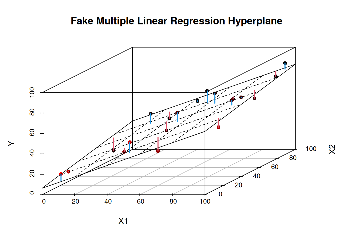
A hyperplane is a higher-dimension version of a line (in 2D) or a plane (in 3D). To illustrate this concept, let’s look at a 3D example with two independent variables.
In this plot:
The points represent our data in 3D space.
The grid represents our fitted hyperplane (which is a plane in this 3D case).
The vertical distances from the points to the plane represent the residuals.
where \(\widehat{\beta}_0\) is the intercept, and \(\widehat{\beta}_1\) and \(\widehat{\beta}_2\) are the coefficients for \(X_1\) and \(X_2\) respectively. We get the \(\widehat\beta\)’s in the same way as we did for simple linear regression: we minimize the sum of the squared residuals (i.e., the sum of the squared vertical distances from the data to the plane).
As we add more predictors, we move beyond three dimensions, and we can no longer visualize the hyperplane. However, the concept remains the same: we’re fitting a flat surface in higher-dimensional space that best approximates our data points according to the least squares criterion. The equation of a hyperplane in \(P + 1\) dimensions (which corresponds to one dependent variables and \(P\) independent variables) we instead have the equation
Just like for simple linear regression, we will estimate the \(\widehat \beta\)’s using the method of least squares. That is, try to minimize the sum of the squared vertical distances from the hyperplane used to fit the data by choosing the \(\widehat \beta\)’s to minimize
7.2.3 Optional: Matrix Representation and a Formula for the Least Squares Estimates
There is a simple expression for the \(\widehat\beta\)’s in multiple linear regression, just like there is for simple linear regression. It is a bit more complicated to explain, however, because it requires matrix/linear algebra to describe. First, we define the following vectors and matricies:
Note that we have included a column of\(1\)’s in the definition of \(\mathbf X\); this will be used to represent the intercept! Now, recall that the we can multiply a matrix with a vector as follows:
(Matrix-vector multiplication is usually taught in high-school Algebra II.)
While complicated up-front, it turns out to be very convenient to use this notation because it makes many expression very simple. For example, the entire model can be rewritten as
\[
\mathbf Y = \mathbf X \boldsymbol \beta + \boldsymbol \epsilon.
\]
Additionally, the sum of squared errors that we need to minimze \(\boldsymbol\beta\) over can be expressed as
\[
(\mathbf Y - \mathbf X \boldsymbol \beta)^\top (\mathbf Y - \mathbf X \boldsymbol\beta)
\]
where the symbol \(\top\) represents the matrix transpose that “flips a matrix on its side”. For example:
where \((\mathbf X^\top \mathbf X)^{-1}\) represents the matrix inverse of the matrix \(\mathbf X^\top \mathbf X\).
7.2.4 Interpreting the Coefficients of the Model
In multiple linear regression, interpreting the coefficients (i.e., the \(\beta\)’s) is a bit more nuanced than in simple linear regression.
Interpretation of the Coefficients
The coefficient \(\widehat \beta_j\) represents the change in the prediction of the dependent variable given a one-unit increase in the corresponding independent variableholding all other variables constant.
This “holding all other variables constant” part is crucial, and is what distinguishes the interpretation of multiple linear regression from simple linear regression.
Let’s use the GPA dataset to illustrate this concept. Consider the following model:
For this dataset, least squares produces the following results:
\(\widehat\beta_{\texttt{hs\_gpa}} = 0.545\);
\(\widehat\beta_{\texttt{sat\_m}} = 0.0155\);
\(\widehat\beta_{\texttt{sat\_v}} = 0.0161\);
\(\widehat\beta_{\texttt{sex}} = -0.142\);
These coefficients can be interpreted as follows:
High school GPA: The estimated coefficient for hs_gpa in this model is 0.545008, which means that if we hold sex and the SAT scores constant that moving from a 3 to a 4 high school GPA increases the predicted GPA by 0.545 grade points.
Sex: The estimated coefficient for sex (which is 1 when the student is male and 0 otherwise; see the section on dummy variables below for how non-numeric predictors like sex are handled) is -0.1418. This means that if two students of different sexes have the same high school GPA and SAT scores, then the male student will have a predicted first year GPA that is 0.1418 points lower than the female student.
SAT Scores: Both sat_m and sat_v have estimated coefficients roughly around 0.015. The units of the SAT scores themselves are in tens of points. This means that increasing the SAT math score of a student (again, holding all else fixed) increases the predicted first year GPA by 0.015 points.
When convenient, we can also consider shifts by more than one point. For example, the estimated coefficient for sat_m being around 0.015 also means that if we increase the SAT math score by 10 units (which corresponds to 100 SAT points) then the predicted GPA goes up by 0.15 points (because \(10 \times 0.015 = 0.15\)).
The intercept (about -0.258) represents the predicted first-year GPA for a student with a high school GPA of 0, SAT scores of 0, and who is female. This isn’t a meaningful prediction in practice, as we don’t have students with 0 GPAs or SAT scores.
7.3 Fitting Multiple Linear Regression in R
We use the same function lm() to fit multiple linear regression as simple linear regression. The code to do this is similar to simple linear regression as well, but we include multiple variables in the formula. The basic recipe looks like this:
## Template code; replace the different parts with your own data and variablesmodel <-lm(dependent_variable ~ independent_variable1 + independent_variable2 + ..., data = dataset)
To illustrate, let’s look at the GPA dataset to predict a students first year GPA based on their high school GPA, SAT math score, SAT verbal score, and sex. Applying the above template, here’s how we fit the model:
In this formula: - fy_gpa is our dependent variable (what we’re trying to predict) - ~ is used to seperate the dependent variable from the independent variables - hs_gpa, sat_m, sat_v, and sex are our independent variables (predictors) - the independent variables are separated by a + - data = fygpa specifies the dataset we’re using
7.3.1 How This Compares to Simple Linear Regression
The glance() function returns quantities whose interpretation does not really change between the simple and multiple linear regression: we have learned about \(R^2\) (r.squared) and \(s\) (sigma) already, and we learn about most of the other entries in this table as we progress through the course.
The tidy() and summary() functions are also mostly the same, with the only change being that we are presented with more than just an intercept and a single slope in the coefficients table: we get a \(\widehat \beta\) for each of the independent variables, and each one has its own standard error, test statistic, and \(P\)-value. We will learn about inference in multiple linear regression next chapter.
7.3.2 Interpreting the Coefficients for the GPA Data
Recall that the coefficients in the output represent the estimated change in the dependent variable for a one-unit increase in the corresponding independent variable, holding all other variables constant. Restating the conclusions we saw earlier:
The estimated coefficient for hs_gpa in this model is 0.545008, which means that if we hold sex and the SAT scores constant that moving from a 3 to a 4 high school GPA increases the predicted GPA by 0.545 grade points.
The estimated coefficient for sexMale (which is 1 when the student is male and 0 otherwise; see the section on dummy variables below for how non-numeric predictors like sex are handled) is -0.1418. This means that if two students of different sexes have the same high school GPA and SAT scores, then the male student will have a predicted first year GPA that is 0.1418 points lower than the female student.
Both sat_m and sat_v have estimated coefficients roughly around 0.015. The units of the SAT scores themselves are in tens of points. This means that increasing the SAT math score of a student (again, holding all else fixed) increases the predicted first year GPA by 0.015 points.
When convenient, we can also consider shifts by more than one point. For example, the estimated coefficient for sat_m being around 0.015 also means that if we increase the SAT math score by 10 units (which corresponds to 100 SAT points) then the predicted GPA goes up by 0.15 points (because \(10 \times 0.015 = 0.15\)).
7.3.3 Using the Model for Prediction
We can also use our fitted model to make predictions for new data:
This will give us the predicted first year GPA for a female student with a 3.8 high school GPA, 650 SAT math score, and 600 SAT verbal score. If we want predictions on the original dataset, we can either not supply the newdata argument (so predict(fygpa_all)) or use the augment() function
For fun, let’s look at the highest possible predicted GPA under this model. This would correspond to a female with a 4.0 GPA and 800 SAT verbal and math scores. This gives
predict(fygpa_all, newdata =data.frame(hs_gpa =4, sex ="Female", sat_m =80, sat_v =80))
1
3.876594
So the ideal student under this model has a predicted first year GPA of 3.88.
7.3.4 Most Things Stay the Same
Going from simple to multiple linear regression introduces some new complexities, but many of the fundamental concepts and quantities remain unchanged. Below we revisit some of the same concepts we defined for simple linear regression, and discuss if necessary how they change when moving from simple to multiple linear regression.
The Predicted Values: To define the fitted values (or predicted values) for the dataset we set
This is the outcome that the model predicts for observation \(i\).
The Residuals: The residuals for the model are defined in the same way as for a simple linear regression:
\[
e_i = Y_i - \widehat Y_i.
\]
Sums of Squares: The decomposition of variability remains unchanged in multiple regression. The total sum of squares (\(\sum_i (Y_i - \bar Y)^2\)) is still partitioned into the regression sum of squares (\(\sum_i (\widehat Y_i - \bar Y)^2\)) and the error sum of squares (\(\sum_i (Y_i - \widehat Y_i)^2\)), such that SST = SSR + SSE. However, in multiple regression, SSR now represents the variability explained by all predictors collectively, rather than a single predictor. Multiple\(R^2\): The multiple \(R^2\) is interpreted just as it was for simple linear regression, except that it now represents the proportion of the variance in the dependent variable explained by all of the independent variables rather than just a single variable. It is not longer the squared correlation between the dependent and independent variable(s) but is instead the squared correlation between \(Y_i\) and \(\widehat Y_i\). The formula for \(R^2\) is still \(R^2 = \text{SSR} / \text{SST} = 1 - \text{SSE}\text{SST}\).
Residual Standard Error: The residual standard error for a multiple linear regression model takes a slightly different form than it does for simple linear regression:
\[
s^2 = \frac{\sum_i e_i^2}{N - P - 1}
\]
where \(P\) is the number of predictors in the model. So, in the case of the GPA dataset, we have \(P = 4\) predictors: sex, high school GPA, and the two SAT scores. We also have 1000 students, so in total the denominator of \(s^2\) will be 995.
More on the Denominator
In general, the denominator of this expression is equal to the number of observations (\(N\)) minus the number of coefficients that we need to estimate (\(P\) coefficients for the \(P\) predictors, and an addition coefficient representing the intercept.) This is useful to know, because it will help us figure out what the correct denominator is in other, more complicated, settings. Remember: the relevant choice of\(P\)in the formula for\(s\)is the number of coefficients that you need to estimate, not the number of independent variables! This is an important distinction to make when using dummy encoding, because a single variable might be associated with more than one coefficient!
7.4 Why Have More Than One Independent Variable?
7.4.1 Better Predictions
Including multiple relevant independent variables often leads to more accurate predictions. Let’s compare the multiple linear regression model (using all variables) to a simple linear regression model (using only high school GPA) for the first-year GPA dataset:
summary(fygpa_all)
Call:
lm(formula = fy_gpa ~ hs_gpa + sat_m + sat_v + sex, data = fygpa)

Residuals:
    Min      1Q  Median      3Q     Max
-2.0601 -0.3478  0.0315  0.4106  1.7042

Coefficients:
             Estimate Std. Error t value Pr(>|t|)
(Intercept) -0.835161   0.148617  -5.620 2.49e-08 ***
hs_gpa       0.545008   0.039505  13.796  < 2e-16 ***
sat_m        0.015513   0.002732   5.678 1.78e-08 ***
sat_v        0.016133   0.002635   6.123 1.32e-09 ***
sexMale     -0.141837   0.040077  -3.539  0.00042 ***
---
Signif. codes:  0 '***' 0.001 '**' 0.01 '*' 0.05 '.' 0.1 ' ' 1

Residual standard error: 0.5908 on 995 degrees of freedom
Multiple R-squared:  0.3666,    Adjusted R-squared:  0.364
F-statistic:   144 on 4 and 995 DF,  p-value: < 2.2e-16
summary(lm(fy_gpa ~ hs_gpa, data = fygpa))
Call:
lm(formula = fy_gpa ~ hs_gpa, data = fygpa)

Residuals:
     Min       1Q   Median       3Q      Max
-2.30544 -0.37417  0.03936  0.41912  1.75240

Coefficients:
            Estimate Std. Error t value Pr(>|t|)
(Intercept)  0.09132    0.11789   0.775    0.439
hs_gpa       0.74314    0.03635  20.447   <2e-16 ***
---
Signif. codes:  0 '***' 0.001 '**' 0.01 '*' 0.05 '.' 0.1 ' ' 1

Residual standard error: 0.6222 on 998 degrees of freedom
Multiple R-squared:  0.2952,    Adjusted R-squared:  0.2945
F-statistic: 418.1 on 1 and 998 DF,  p-value: < 2.2e-16
We note make two observations based on the above results:
The multiple R-squared value is increases substantially when using more predictors; whereas before we accounted for only 29.5% of the variance, we now account for 36.6% of the variance, an increase of around 7%. While directly comparing R-squared across models is a somewhat subtle issue (which we will discuss in future chapters), this indicates that themodel with multiple predictors explains substantially more of the variance in first year GPA.
The residual standard error is lower for the multiple for the multiple linear regression model; rather than being off, on average, by 0.622 grade points in either direction, we are off by 0.59 grade points.
Practically speaking, these differences are modest and so, depending on my specific aims, I might use the simple linear regression or multiple linear regression. As someone who is involved in admissions it is interesting (to me) that high school GPA is already a very good proxy for academic performance and that SAT scores contribute only modestly beyond that.
7.4.2 Controlling for Possible Confounders
Another crucial reason for including multiple independent variables is to control for confounding factors. A confounder is a variable that influences both the dependent and independent variables, potentially leading to misleading conclusions.
For example, let’s revisit the wage gap data example given at the start of this chapter. The wage gap between men and women has been pointed to as a problem that can be addressed via sex discrimination policy, the idea being that employers are discriminating against women on the basis of their gender when they pay them less. Whether such a policy seems desirable or not, from the perspective of the regression, depends critically on whether we control for additional factors. For example, we might run a regression that looks like this:
simple_model <-lm(wage ~ sex, data = wage_data)
and conclude from a large sex coefficient that it addressing the wage gap could be handled via anti-discrimination measures in the workplace. A more comprehensive model might instead look like this:
full_model <-lm(wage ~ sex + education + experience + occupation + industry, data = wage_data)
The results from this model could paint a more nuanced picture, and suggest different policy recommendations:
Direct Discrimination: The coefficient for ‘sex’ now represents the wage gap that exists even when other factors are held constant. This could inform policies targeting explicit gender-based discrimination.
Educational Differences: If education significantly predicts wages, policies might focus on ensuring equal access to education and encouraging women to enter high-paying fields of study.
Work Experience Gap: If experience is a major factor, policies might address issues like parental leave and child care to help women maintain continuous workforce participation.
Occupational Segregation: Large coefficients for occupation or industry might suggest policies to encourage gender diversity across all sectors and address why certain high-paying fields are male-dominated.
A General Comment on Sex Discrimination and the Wage Gap
Generally speaking, I advise against interpreting the above discussion as arguments in favor or against the claim that a wage gap is justified from a fairness perspective. The more nuanced version of the “no” argument, rather than relying on sex discrimination at the hiring stage, is that the wage gap results from a “leaky pipeline” that funnels women out of high-paying jobs as they move through the education system, and that (if we wanted to fix it) policy should focus on ensuring that women are encouraged to stay in the pipeline to higher paying jobs.
7.5 Non-Numeric Predictors
Datasets that we encounter often have variables that are not numeric but rather categorical in nature; that is, rather than taking numeric values (0, 1, 2, etc) they take non-numeric values (“red”, “blue”, “green”, etc) where their values do not possess a natural ordering. Examples of this in the datasets we have considered are marital status in the wages dataset (married, divorced, single, etc.) or plant species in the iris dataset (setosa, virginica, versicolor).
While these categorical variables can contain valuable information (occupation is very predictive of wage, iris species is highly predictive of sepal length and width, etc.), regression models require numeric inputs. So how do we incorporate these non-numeric predictors into a linear regression model?
7.5.1 The Prestige Dataset
We’ll be using the Prestige dataset from the car package. This dataset contains information about various occupations, including their “prestige scores” and characterstics. Let’s take a look at the data:
## Install and load the car package if you haven't alreadylibrary(car)data(Prestige)# View the first few rows and structure of the datasethead(Prestige)
prestige is the prestige score of the occupation (our dependent variable)
education is the average education level (years) for the occupation
income is the average income for the occupation
women is the percentage of women in the occupation
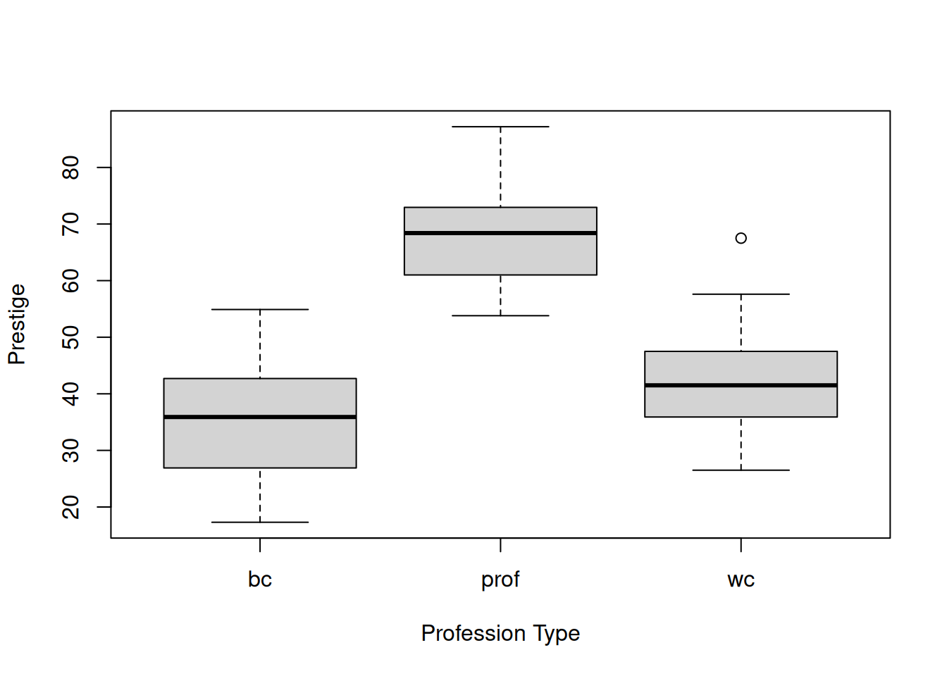
type is the type of occupation (bc, prof, or wc for blue-collar, professional, and white-collar respectively)
The type variable is a categorical predictor, taking three levels (blue-collar, professional, or white-collar). A boxplot that quickly visualizes the relationship between type and prestige is given below:
Dummy variable encoding allows us to represent categorical variables in terms of binary (0 or 1) variables that can be included as numeric variables in our regression model.
Here’s how it works:
For a categorical variable with \(k\) categories, we create \(k - 1\) new binary variables; in the context of the Prestige data, \(k = 3\) (for the different levels of type), so we need \(3 - 1 = 2\) new binary variables. These variables are referred to as dummy variables.
Each of these new variables represents one of the new categories. So, for example, for the Prestige dataset, we create a variable typeprof that is 1 if the occupation is professional and 0 otherwise, and a variable typewc that is 1 if the occupation is white-collar and 0 otherwise.
For the category that is not assigned a dummy variable (in this case, the blue-collar, or bctype) we know that the occupation is of this type if both typeprof and typewc are both zero. This level is called the reference level, and it plays an important role in interpreting the meaning of the variables
We can use non-numeric variables like type in a linear regression using the lm function just like we would with a numeric variable. So, for example, we can predict prestige using just the variable type as follows:
prestige_lm <-lm(prestige ~ type, data = Prestige)
Now, let’s look at the output using the tidy function:
Rather than having a single coefficient for type, we instead have the two dummy variables. Notice that R takes care of the construction of the dummy variables for you; it has automatically made blue-collar the reference category and made dummy variables for the profession and white-collar types. In this case, it chose to make blue-collar the reference category because bc comes before prof and wc alphabetically.
7.5.3 Interpreting Dummy Variables
To see how to interpret the dummy variables, let’s write out explicitly what the model is for prestige:
Considering the different occupation types separately:
For professional occupations, the model predicts \(\beta_0 + \beta_1\) since \(\texttt{typeprof} = 1\) and \(\texttt{typewc} = 0\).
For white color occupations, the model predicts \(\beta_0 + \beta_2\) since \(\texttt{typeprof} = 0\) and \(\texttt{typewc} = 1\).
For blue collar occupations, the model predicts \(\beta_0\) since \(\texttt{typeprof} = 0\) and \(\texttt{typewc} = 0\).
We can conclude that:
The intercept represents the average prestige score for the reference category.
The coefficients for typeprof and typewc represent the difference in average prestige score for professional and white-collar occupations compared to blue-collar occupations, respectively.
Interpreting the Coefficients
In general, we can interpret the coefficients of the non-reference categories as the difference in the average value of the independent variable for observations at the associated level and the observations at the reference level. So, the estimate of 32.321 for the typeprof variable implies that professional occupations have a predicted prestige score 32.321 points higher than blue collar occupations; similarly, white collar occupations have a predicted prestige score 6.716 points higher than blue collar occupations.
7.5.4 Multiple Predictors Including Categorical Variables
Now, let’s include both numeric and categorical predictors in our model:
prestige_lm_full <-lm(prestige ~ education + income + women + type, data = Prestige)summary(prestige_lm_full)
Call:
lm(formula = prestige ~ education + income + women + type, data = Prestige)

Residuals:
     Min       1Q   Median       3Q      Max
-14.7485  -4.4817   0.3119   5.2478  18.4978

Coefficients:
              Estimate Std. Error t value Pr(>|t|)
(Intercept) -0.8139032  5.3311558  -0.153 0.878994
education    3.6623557  0.6458300   5.671 1.63e-07 ***
income       0.0010428  0.0002623   3.976 0.000139 ***
women        0.0064434  0.0303781   0.212 0.832494
typeprof     5.9051970  3.9377001   1.500 0.137127
typewc      -2.9170720  2.6653961  -1.094 0.276626
---
Signif. codes:  0 '***' 0.001 '**' 0.01 '*' 0.05 '.' 0.1 ' ' 1

Residual standard error: 7.132 on 92 degrees of freedom
  (4 observations deleted due to missingness)
Multiple R-squared:  0.8349,    Adjusted R-squared:  0.826
F-statistic: 93.07 on 5 and 92 DF,  p-value: < 2.2e-16
Interpreting the results:
The intercept represents the average prestige score for blue-collar occupations when all other variables are zero (which may not be meaningful in this context).
The coefficients for education, income, and women represent the change in predicted prestige score for a one-unit increase in each of these variables, holding other variables constant.
The coefficients for typeprof and typewc represent the difference in predicted prestige score for professional and white-collar occupations compared to blue-collar occupations, respectively, when all other variables are held constant.
7.6 Exercises
7.6.1 Exercise 1: Boston Housing Revisited
This exercise explores the Boston Housing dataset again, this time using multiple linear regression. First, load the data by running this command:
Boston <- MASS::Boston
and re-familiarize yourself with the contents of the dataset by running ?MASS::Boston.
Create a multiple linear regression model to predict medv (median house value) using rm (the average number of rooms), lstat (proportion of “lower status” individuals in the tract), crim (per capita crime rate) and nox (nitric oxide concentration). What is the R-squared associated with this model? Interpret it.
Interpret each of the coefficients in the model.
Compare the R-squared of this multiple regression model to simple linear regression models that use each predictor individually. What do you observe?
Use the augment() function from the broom package to add fitted values and residuals to your dataset. For the first three suburbs listed, interpret the fitted values and residuals.
Use the fitted model to predict the median home value in a tract with the six average rooms, 8% lower status individuals, a crime rate of 0.22, and nitric oxide concentration of 0.585.
7.6.2 Exercise 2: Affairs Revisited
This exercise revisits the Affairs dataset to look at multiple factors and see to what extent they predict the occurence of extra-marital affairs. First, load the data by running
library(AER)data("Affairs")
Descriptions for each of the variables can be obtained by running ?Affairs.
Create a multiple linear regression model to predict the number of affairs using all of the other variables in the dataset. Use the lm() function and store the result in affairs_model.
Use the summary() function to view the results of your model. Interpret the coefficients for gender, age, children, and religiousness.
What is the R-squared value of this model? Interpret what this means in the context of explaining the variability in the number of affairs.
Use the augment() function from the broom package to add fitted values and residuals to your dataset. For the first three individuals listed, interpret the fitted values and residuals.
Based on the model, give your rough impression of how each of the variables relates to the affair frequency. What sorts of individuals tend to have larger affair frequencies? What sorts tend to have smaller affair frequencies?
Fit a multiple linear regression model predicting sales using all three advertising mediums (TV, radio, and newspaper).
Interpret each coefficient in your model. Which advertising medium appears to be most effective?
Compare the R-squared of this model to the R-squared of the simple linear regression model using only TV advertising. How much additional variance is explained by including radio and newspaper?
Use your model to predict sales for a product with the following advertising budgets: TV: $200,000, Radio: $80,000, Newspaper: $50,000.
What is the residual standard error? Interpret it within the context of this problem.
7.6.4 Exercise 4: Wage Data Regression Analysis
We revisit the wages dataset, which we can load as follows:
Fit a linear regression that predicts wage using hours, IQ, education level, experience, job tenure, age, marital status, urban/rural status, number of siblings, birth order, mothers education level, and fathers education level. Then, print a summary of the results using summary().
Interpret the coefficients for IQ, education (educ), and experience (exper). What does each coefficient represent in the context of predicting wages?
Interpret the coefficients for the categorical variables ‘married’ and ‘urban’. How do these factors appear to influence wages?
Calculate and interpret the predicted difference in wages between:
A married person living in an urban area versus an unmarried person living in a rural area (assuming all other variables are held constant)
Two individuals who differ by 5 years of education but are identical on all other measured variables
What is the R-squared value of this model, and how does it compare to the R-squared in a model that only controls for IQ and age? Interpret what this means in the context of explaining wage variability.
What is the residual standard error of the model? Interpret this value in the context of predicting wages.
The intercept of this model is negative. Interpret what this means and discuss whether this interpretation is meaningful in the real world.