This chapter discusses some other issues that arise when building a linear regression model. First we discuss the issue of multicollinearity, which occurs when some of the independent variables are (almost) redundant with each other. We then discuss how to think through which variables we should (or should not) include in a regression when our goal is to establish a causal relationship.
14.1 Multicollinearity
One issue that can arise when building linear regression models is multicollinearity. This occurs when at least one of the independent variables \(X_{ij}\) can be predicted using the other \(X_{ij}\)’s extremely well; the worst case of this is a violation of the full rank assumption, which occurs when one variable can be predicted exactly from the others. In other words, multicollinearity occurs when there exist very strong correlations among the independent variables.
The main issue caused by multicollinearity is that if (say) \(X_{i1}\) and \(X_{i2}\) are highly correlated, then it can be difficult to tell whether a change in \(y_i\) is due to \(X_{i1}\) changing or is due to \(X_{i2}\) changing, because in the data they will typically change together. We first look at some examples.
14.1.1 Extreme Example: GPA Dataset
To illustrate the issue in as dramatic a fashion as possible, let’s see what happens with the GPA dataset if we include all three of sat_m, sat_v, and sat_sum as independent variables when trying to predict first year GPA on the GPA dataset:
fygpa <-read.csv("https://raw.githubusercontent.com/theodds/SDS-348/master/satgpa.csv")fygpa$sex <-ifelse(fygpa$sex ==1, "Male", "Female")fygpa_all <-lm(hs_gpa ~ sex + sat_v + sat_m + sat_sum, data = fygpa)summary(fygpa_all)
Call:
lm(formula = hs_gpa ~ sex + sat_v + sat_m + sat_sum, data = fygpa)

Residuals:
     Min       1Q   Median       3Q      Max
-1.36117 -0.34298  0.01838  0.35353  1.89917

Coefficients: (1 not defined because of singularities)
             Estimate Std. Error t value Pr(>|t|)
(Intercept)  1.469428   0.109734  13.391  < 2e-16 ***
sexMale     -0.254400   0.031118  -8.175 8.92e-16 ***
sat_v        0.013845   0.002067   6.697 3.55e-11 ***
sat_m        0.021739   0.002080  10.450  < 2e-16 ***
sat_sum            NA         NA      NA       NA
---
Signif. codes:  0 '***' 0.001 '**' 0.01 '*' 0.05 '.' 0.1 ' ' 1

Residual standard error: 0.4738 on 996 degrees of freedom
Multiple R-squared:  0.237, Adjusted R-squared:  0.2347
F-statistic: 103.1 on 3 and 996 DF,  p-value: < 2.2e-16
In the above output, we see that the model more-or-less refused to do anything with sat_sum! Rather than reporting estimated coefficients or \(P\)-values, the model simply removes sat_sum from the model. This is because sat_sum is perfectly predicted by sat_v + sat_m, and so is an extreme instance of multicollinearity.
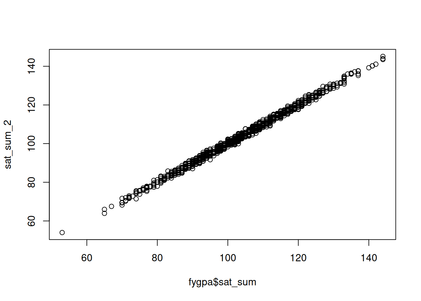
To make things a bit less extreme, below I create a new variable sat_sum_2 that is almost equal to sat_sum but with a little bit of noise added in so that it is no longer perfectly predicted by sat_m + sat_v:
## Set the random number seed so that results can be reproducedset.seed(12039)## Make a new variable that adds an additional, normally distributed, errorsat_sum_2 <- fygpa$sat_sum +rnorm(n =nrow(fygpa), mean =0, sd =1)## Plot the old SAT total score against the modified oneplot(fygpa$sat_sum, sat_sum_2)
Now, let’s see what happens if we use sat_sum_2 as an independent variable along with sat_m and sat_v which predict it nearly perfectly:
fygpa_all_2 <-lm(hs_gpa ~ sex + sat_v + sat_m + sat_sum_2, data = fygpa)summary(fygpa_all_2)
Call:
lm(formula = hs_gpa ~ sex + sat_v + sat_m + sat_sum_2, data = fygpa)

Residuals:
     Min       1Q   Median       3Q      Max
-1.36254 -0.34224  0.01715  0.35524  1.89917

Coefficients:
            Estimate Std. Error t value Pr(>|t|)
(Intercept)  1.46942    0.10979  13.384  < 2e-16 ***
sexMale     -0.25438    0.03113  -8.170 9.28e-16 ***
sat_v        0.01558    0.01483   1.050    0.294
sat_m        0.02345    0.01463   1.602    0.109
sat_sum_2   -0.00172    0.01458  -0.118    0.906
---
Signif. codes:  0 '***' 0.001 '**' 0.01 '*' 0.05 '.' 0.1 ' ' 1

Residual standard error: 0.4741 on 995 degrees of freedom
Multiple R-squared:  0.237, Adjusted R-squared:  0.2339
F-statistic: 77.27 on 4 and 995 DF,  p-value: < 2.2e-16
After adding the redundant variable sat_sum_2 we see that now all of the SAT scores appear to not be significant!
The Consequences of Multicollinearity
Multicollinearity is problematic for a couple of different reasons:
It tends to increase the standard errors of our regression coefficients, i.e., it makes our estimates less precise. The standard errors of sat_v and sat_m are, for example, more than 7 times larger than they are when sat_sum_2 is excluded.
Because of this, it makes existing effects appear less significant than they otherwise would be.
14.1.2 Less Extreme Example: Wages Dataset
For a more realistic example of multicollinearity, we will revisit the wages dataset, which contains information on the weekly wages of individuals in the 1980s, along with some other personal attributes:
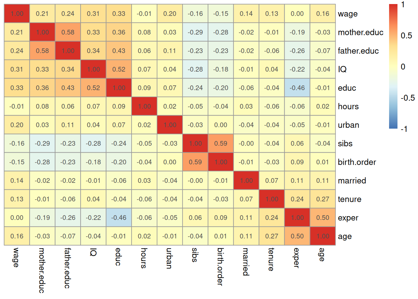
A quick (but imperfect) way to try to detect multicollinearity is to look at the correlation matrix of the data. The correlation matrix, constructed with the cor() function, makes a matrix \(R\) such that the \((j,k)^{\text{th}}\) element of \(R\) is given by the correlation between \(X_{ij}\) and \(X_{ik}\). We can get the correlation matrix for the wages dataset as follows:
correlation_matrix <-cor(wages, use ="pairwise.complete.obs")print(correlation_matrix)
Reading the above figure, we see (for example) that the correlation between sibs and birth.order is \(0.59\), while (for example) the correlation between IQ and sibs is \(-0.24\).
From the correlation matrix, we can see that educational attainment and IQ are highly correlated with each other. This has rather tangible effects on the inferences we would get for the effect of education. If we fit a model using only education and IQ, we get the following results:
wage_lm <-lm(log(wage) ~ educ + IQ, data = wages)summary(wage_lm)
Call:
lm(formula = log(wage) ~ educ + IQ, data = wages)

Residuals:
     Min       1Q   Median       3Q      Max
-2.01601 -0.24367  0.03359  0.27960  1.23783

Coefficients:
             Estimate Std. Error t value Pr(>|t|)
(Intercept) 5.6582876  0.0962408  58.793  < 2e-16 ***
educ        0.0391199  0.0068382   5.721 1.43e-08 ***
IQ          0.0058631  0.0009979   5.875 5.87e-09 ***
---
Signif. codes:  0 '***' 0.001 '**' 0.01 '*' 0.05 '.' 0.1 ' ' 1

Residual standard error: 0.3933 on 932 degrees of freedom
Multiple R-squared:  0.1297,    Adjusted R-squared:  0.1278
F-statistic: 69.42 on 2 and 932 DF,  p-value: < 2.2e-16
whereas if we only use education we obtain
wage_lm_educ <-lm(log(wage) ~ educ, data = wages)summary(wage_lm_educ)
Call:
lm(formula = log(wage) ~ educ, data = wages)

Residuals:
     Min       1Q   Median       3Q      Max
-1.94620 -0.24832  0.03507  0.27440  1.28106

Coefficients:
            Estimate Std. Error t value Pr(>|t|)
(Intercept) 5.973062   0.081374   73.40   <2e-16 ***
educ        0.059839   0.005963   10.04   <2e-16 ***
---
Signif. codes:  0 '***' 0.001 '**' 0.01 '*' 0.05 '.' 0.1 ' ' 1

Residual standard error: 0.4003 on 933 degrees of freedom
Multiple R-squared:  0.09742,   Adjusted R-squared:  0.09645
F-statistic: 100.7 on 1 and 933 DF,  p-value: < 2.2e-16
We see that including IQ in the model makes the evidence for the effect of education just a tad smaller: while still highly significant, the \(T\)-statistic for education decreases from 10 to 5 if we include IQ. We can contrast this with what happens if we use a model that includes age (which is not highly correlated with educ) instead of IQ:
wage_age_educ <-lm(log(wage) ~ age + educ, data = wages)summary(wage_age_educ)
Call:
lm(formula = log(wage) ~ age + educ, data = wages)

Residuals:
     Min       1Q   Median       3Q      Max
-1.85403 -0.23538  0.02986  0.26911  1.37285

Coefficients:
            Estimate Std. Error t value Pr(>|t|)
(Intercept) 5.225153   0.159896  32.679  < 2e-16 ***
age         0.022450   0.004153   5.406 8.18e-08 ***
educ        0.060228   0.005875  10.251  < 2e-16 ***
---
Signif. codes:  0 '***' 0.001 '**' 0.01 '*' 0.05 '.' 0.1 ' ' 1

Residual standard error: 0.3944 on 932 degrees of freedom
Multiple R-squared:  0.1249,    Adjusted R-squared:  0.123
F-statistic: 66.49 on 2 and 932 DF,  p-value: < 2.2e-16
In this case, age basically doesn’t change anything about the effect of educ: the \(T\)-statistic is in fact slightly higher when age is included.
Summarizing What We’ve Seen
The above examples show that multicollinearity, i.e., large correlations among the independent variables can result in less precise estimates. Specifically, multicollinearity tends to drive up the standard errors, which leads to smaller \(T\)-statistics, all other things being equal.
14.1.3 Measuring Multicollinearity with Variance Inflation Factors
Correlation matrices can help us visually detect multicollinearity, but we might want a more precise, quantitative, measure. The Variance Inflation Factor (VIF) provides this. For each predictor variable \(X_{ij}\), its VIF tells us how much of the standard error of that regression coefficient is increased due to multicollinearity with the other variables. It is defined to be:
\[
\text{VIF}_j = \frac{1}{1 - R^2_j}
\]
where \(R^2_j\) is the R-squared we would get if we fit a linear regression with \(X_{ij}\) as the dependent variable and used the other independent variables as independent variables.
What the VIF Represents
With a bit of math, it can be shown that the VIF tells us the factor by which the variance of \(\widehat{\beta}_j\) is increased compared to what it would be if \(X_{ij}\) were uncorrelated with other predictors. For example, if \(VIF_j = 4\), then the standard error of \(\widehat{\beta}_j\) is twice as large as it would be in the absence of multicollinearity (since \(\sqrt{4}=2\)).
To calculate the VIF for variable \(j\), we:
Regress variable \(j\) on all other predictors in the model
Calculate \(R^2_j\) from this regression
Compute \(VIF_j = \frac{1}{1-R^2_j}\)
Intuitively, the idea is that if \(X_{ij}\) can be predicted extremely well by the other variables, then \(R^2_j\) will be close to \(1\), making the VIF very large. Conversely, if \(X_j\) is uncorrelated with other predictors, \(R^2_j\) will be close to 0, giving a VIF close to 1.
The R function vif() from the car package calculates VIFs automatically:
library(car)vif(wage_lm)
    educ       IQ
1.362293 1.362293
When is the VIF Large?
As a rule of thumb, VIF values greater than 5 or 10 indicate problematic multicollinearity. However, these thresholds aren’t universal; it is possible to have very high VIFs without necessarily needing to modify an analysis.
We can also try this out with our GPA dataset:
vif(fygpa_all_2)
       sex      sat_v      sat_m  sat_sum_2
  1.077151  66.294590  67.968657 194.029650
We see once again that the VIF for sat_sum is extremely high, indicating problematic multicollinearity.
14.1.4 What to Do About Multicollinearity
Upon finding multicollinearity, there are several paths we can take. The list below is inspired by these slides:
Do nothing. Sometimes the best course of action is to simply acknowledge the presence of multicollinearity and proceed with your analysis. If your results are highly significant anyway, then it doesn’t really matter much that multicollinearity is increasing the standard errors of the regression coefficients. For example, in the wages dataset, we would not want to remove either education or IQ: if we want to know the effect of education on its own, then it is probably important to control for IQ precisely because it is correlated with education.
Additionally, if your primary goal is prediction rather than inference about individual coefficients, multicollinearity may not seriously impair your model’s usefulness. The predictions will still be accurate (as long as you aren’t extrapolating); only the individual coefficient estimates and their standard errors are affected.
Remove One or More Variables. If, as with the GPA dataset, some variables are truly redundant, then we can remove them guilt-free. A high degree of multicollinearity may indicate we are “measuring the same thing twice” and we might drop one of the variables to fix this. The choice of which variable to drop should be guided by theory rather than purely statistical considerations.
For instance, poverty level and income are often given in governmental surveys, but these variables are highly correlated and contain essentially the same information; most of the time, people just include poverty level.
For another example, suppose I am interested in predicting someone’s intelligence from their hand size. If I control for both the size of someone’s left hand and their right hand, then I should expect a lot of multicollinearity because these two variables are essentially measuring the same thing. Instead, I could include one hand only or average the two hand sizes together.
Transform or Combine Variables. Sometimes multicollinearity can be addressed through clever respecification of the model. Rather than including closely related variables separately, you might combine them in a meaningful way. For example, in macroeconomic models, using GDP per capita \((GDP/Population)\) instead of including GDP and population separately often makes both theoretical and statistical sense.
Collect More Data. While not always feasible, increasing sample size will improve the precision of your estimates and can help mitigate the practical consequences of multicollinearity. The underlying correlations between variables won’t change, but larger samples provide more information to help distinguish their separate effects. However, collecting additional data is often expensive or impossible, so this solution may not be practical.
14.2 Other Factors in What to Include
A more subtle aspect of model selection is that we should carefully choose our models so that they answer the scientific questions we are interested in. While statistical measures like R-squared, \(P\)-values, and VIFs provide important technical guidance, the choice of variables to include or exclude should be driven primarily by the research objectives and what we hope to learn from the data.
14.2.1 Omitted Variable Bias: Control for Common Causes
In many research problems we don’t aim just to determine an association between the dependent variable and independent variable(s), but to establish a causal relation. That is, we might like to (for example) conclude that pursuing higher education causes one’s income to increase on average.
An in-depth treatment of causal inference is beyond the scope of this course, however, a prerequisite for a slope \(\beta_j\) to have a causal interpretation is that we control for all common causes of \(Y_i\) and \(X_{ij}\). Common causes are also referred to as confounders, and failure to include all confounders in a regression can lead to omitted variable bias. For example, in understanding the relationship between education and wages:
Age might be a confounder since it affects both education level (older people had different educational opportunities) and wages (older people have more work experience).
Family background could influence both educational attainment and wage-earning potential; a common indicator of socio-economic status that we have access to is the educational attainment of an individual’s parents.
Individuals with higher IQs might be both more likely to have higher educational attainment and also have higher wages.
Because these are all common causes of educational attainment and wages, it is appropriate to include all of these variables in the wages model, and in my opinion this should be done regardless of what their \(P\)-values are or what any model selection procedure might tell you. As shown below, the decision to include these variables also very directly influences the size of the education effect we find:
summary(lm(wage ~ educ, data = wages))
Call:
lm(formula = wage ~ educ, data = wages)

Residuals:
    Min      1Q  Median      3Q     Max
-877.38 -268.63  -38.38  207.05 2148.26

Coefficients:
            Estimate Std. Error t value Pr(>|t|)
(Intercept)  146.952     77.715   1.891   0.0589 .
educ          60.214      5.695  10.573   <2e-16 ***
---
Signif. codes:  0 '***' 0.001 '**' 0.01 '*' 0.05 '.' 0.1 ' ' 1

Residual standard error: 382.3 on 933 degrees of freedom
Multiple R-squared:  0.107, Adjusted R-squared:  0.106
F-statistic: 111.8 on 1 and 933 DF,  p-value: < 2.2e-16
summary(lm(wage ~ educ + age + IQ + mother.educ, data = wages))
Call:
lm(formula = wage ~ educ + age + IQ + mother.educ, data = wages)

Residuals:
    Min      1Q  Median      3Q     Max
-809.23 -244.97  -37.92  190.94 2176.18

Coefficients:
            Estimate Std. Error t value Pr(>|t|)
(Intercept) -927.735    167.294  -5.546 3.91e-08 ***
educ          36.621      6.957   5.264 1.79e-07 ***
age           22.718      4.121   5.513 4.68e-08 ***
IQ             5.126      1.005   5.100 4.18e-07 ***
mother.educ   12.177      4.865   2.503   0.0125 *
---
Signif. codes:  0 '***' 0.001 '**' 0.01 '*' 0.05 '.' 0.1 ' ' 1

Residual standard error: 371.4 on 852 degrees of freedom
  (78 observations deleted due to missingness)
Multiple R-squared:  0.1721,    Adjusted R-squared:  0.1682
F-statistic: 44.29 on 4 and 852 DF,  p-value: < 2.2e-16
While education is still relevant, we find that much of its effect can alternately be explained by the other variables (with the estimated slope cut from 60.2 to 36.6).
14.2.2 Overcontrol Bias: You Might Not Want to Control for Everything
While omitted variable bias concerns bias that occurs due to failing to include a variable, overcontrol bias occurs when bias results from including variables that we shouldn’t. Suppose, for example, that we are interested in the effect of the drug semaglutide (also known as Ozempic) on diabetes symptom severity. Specifically, suppose we have the following question:
For a given person with type II diabetes, how much improvement in their symptoms should they expect if they start taking semaglutide?
For this objective controlling for weight loss in our analysis would be a mistake. If we control for weight loss in our regression, we’re essentially asking “What is the effect of Ozempic on diabetes symptoms, holding weight constant?” — but this removes one of the primary pathways through which the drug works! In other words, a large part of the reason Ozempic is effective at treating diabetes is that it causes weight loss, so if we control for weight loss then Ozempic will look less effective than it actually is.
This illustrates a key principle: if we are interested in the total effect of a clinical treatment on some outcome, we should not control for other variables (also called mediators) that are themselves affected by the treatment. The causal chain in this example is:
By controlling for weight loss, we would dramatically underestimate the drug’s effectiveness, since we’d only be measuring the direct effects of the drug that don’t operate through weight loss. This would be misleading if we’re interested in the total effect of Ozempic on diabetes symptoms.
This same principle applies in many other contexts:
When studying the effect of exercise on cardiovascular health, we shouldn’t control for blood pressure reduction.
When analyzing the impact of education on income, we shouldn’t control for job title.
When examining the effect of study time on college admission, we shouldn’t control for test scores.
In each case, controlling for these intermediate variables would mask important pathways through which the treatment affects the outcome, leading to biased estimates of the total effect we’re trying to measure.
14.2.3 Another Reason Not To Trust Automatic Model Selection
In Chapter 13 we discussed how automatic model selection procedures like stepwise regression can be unreliable for statistical reasons - they can capitalize on chance patterns in the data and produce overconfident \(P\)-values. The concepts of confounding and overcontrol bias provide even more fundamental reasons to be skeptical of automatic selection methods.
Consider how stepwise regression typically works: it adds or removes variables based on statistical criteria like AIC. However, these metrics know nothing about the causal structure of our problem! This leads to several serious issues:
Confounding Bias: Automatic selection might drop important confounding variables just because they don’t have a “significant” relationship with the outcome. For example, in studying Ozempic’s effect on diabetes, stepwise regression might drop “access to healthcare” if it’s only weakly correlated with symptoms. But if access to healthcare influences both who gets Ozempic and how well their diabetes is managed, excluding it leads to confounding bias. The statistical insignificance of a confounder doesn’t make the confounding go away!
Overcontrol Bias: Conversely, automatic selection might include mediator variables just because they’re strongly correlated with the outcome. For instance, when studying Ozempic’s effects, stepwise regression would likely include weight loss because it’s strongly related to diabetes symptoms. But as we discussed earlier, this controls away one of the main ways through which Ozempic works. The strong statistical relationship is precisely because it’s a mediator we shouldn’t control for!
It is for these reasons that I do not particularly like automatic model selection. It is possible to fix the post-selection inference problems using data splitting, but the above flaws with automatic model selection are fundamental when the purpose of the analysis is to draw causal conclusions.
14.3 Exercises
14.3.1 Exercise: Boston Housing
The following problem revisits the Boston housing dataset, where our interest is in understanding the relationship between the concentration of nitrous oxide in a census tract (nox) and the median home value in that tract. First, we load the data:
We will only look at a subset of the variables in Boston; the following code removes the variables we are not interested in:
boston_sub <-select(Boston, -zn, -chas)
Use the cor function to get the correlation matrix for the boston_sub dataset and store the result in a variable called boston_cor. Print the output and then state what the different entries in the result correspond to; why are there 1’s on the “diagonal” of the matrix?
The pheatmap function in the pheatmap package is useful for visualizing things like correlation matrices. After doing part (a), run the following code after uncommenting the lines:
Explain what is displayed in the figure. What variable is most strongly positively associated with medv? Negatively?
Based on the plot from the previous question, which pair of variables appear to have the highest correlation?
Fit a model predicting medv from the variables nox, lstat, age, dis, rad, black, tax, and ptratio (store the result in a variable boston_lm). Report the multiple \(R^2\) and the estimate of the standard deviation \(\sigma\) of the errors.
Run library(car) to load the car package (install the package if needed) and then use the vif function to compute the variance inflation factors (VIFs) for the different predictors. Are any of the VIFs concerning?
Fit a new model that removes the variables with high VIFs and compare the summary of this model with that of the original. In terms of \(R^2\), the residual standard deviation, and the variables that the model has found to be statistically significant, what has changed? Would you prefer the model with or without the high VIF variables (no right answers here, just think carefully about whether having a high VIF alone would warrant removing a variable)?
Some researchers observed — notice the choice of word! — the following data on 20 individuals with high blood pressure.
The researchers were interested in determining if a relationship exists between blood pressure and age, weight, body surface area, duration, pulse rate and/or stress level.
The columns of this dataset are given below:
BP: blood pressure (in mm Hg)
Age: age (in years)
Weight: weight (in kg)
BSA: body surface area (in sq m)
Dur: length of time patient has had hypertension (in years)
The scientific interest was to determine which of the variables are predictive of blood pressure, and to what extent.
Visualize the correlation matrix by first using cor to compute the correlation matrix and then using the pheatmap function on the result. Based on the results, would you guess that multicollinearity will be an issue? Why?
## Make pheatmap: uncomment to run the code, make sure to create the ## correlation matrix first# pheatmap(bp_cor,# treeheight_col = 0,# treeheight_row = 0,# display_numbers = TRUE,# breaks = seq(-1, 1, length = 101))
Fit a linear model predicting BP from the other variables. Which variables in this model are statistically significant at the \(0.05\) significance level, assuming that all of the other variables are included in the model?
Use the vif function in the car package to compute the variance inflation factors (VIFs), saving the results to a variable vif_bp. Then, make a barplot showing the VIFs. Based on the results, which variables have concerningly-high VIFs?
Fit a new model with Weight removed. Does the significance of any of the remaining variables drastically change?
In part (d) you should have found that Age became less statistically significant while BSA became more statistically significant. Based on the correlation matrix from part (a), explain practically why BSA went from being marginally significant to being highly statistically significant.
Why did Age become less significant? Explain your answer in terms of the reduction in residual standard error provided by including Weight (i.e., including Weight makes the** estimated\(\sigma\) **much smaller).