my_sin_data <- read.csv("https://raw.githubusercontent.com/theodds/SDS-348/refs/heads/master/sin_data.csv",
header = TRUE)13 Model Evaluation and Selection
Throughout this course, we have often analyzed the same dataset using multiple different models. The goal of this chapter is to try to provide guidance on how to decide which model, of potentially many different models, we should use.
13.1 Example: Fitting A Sine Curve
In Chapter 11 we saw that linear regression was up to the task of fitting non-linear relationships such as a sine curve:
\[ Y_i = \sin(2 \, \pi\, X_i) + \epsilon_i. \]
We can load some artificial data I created with the following command:
and then plot the data:
plot(my_sin_data$x, my_sin_data$y)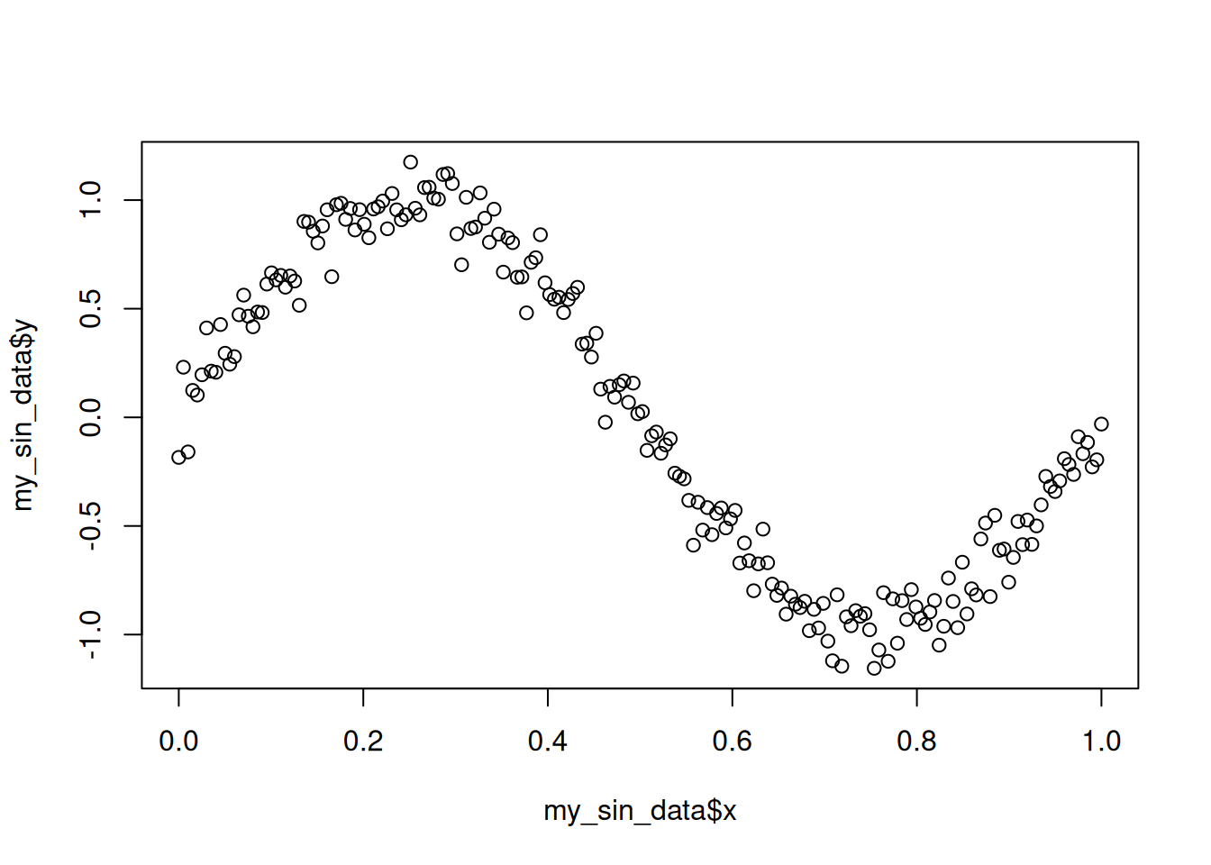
The way we handled nonlinear relationships was to notice that we can approximate essentially any smooth relationship between \(X_i\) and \(Y_i\) using a polynomial expansion:
\[ Y_i \approx \beta_0 + \beta_1 \, X_i + \beta_2 \, X_i^2 + \cdots + \beta_B \, X_i^B + \epsilon. \]
So we can get a decent fit to the relationship between \(X_i\) and \(Y_i\) by fitting some polynomial models. For example, to fit a third degree polynomial (i.e., a cubic) using lm() we can do the following:
poly_lm <- lm(y ~ poly(x, 3), data = my_sin_data)Here is what we get with a third-degree polynomial:
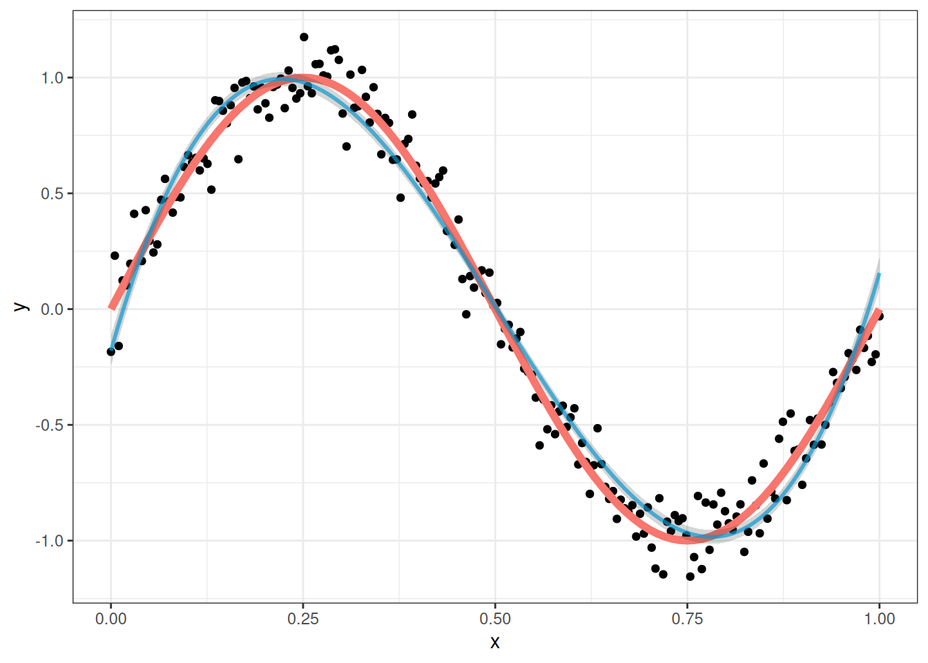
The blue line above is the fit of our regression while the red line is the true relationship, and the band around the blue line is a 95% confidence interval for the line.
This seems to work pretty well, but this invites the obvious question: why stop at a third degree polynomial? While the fit is pretty good, we see that the 95% bands actually do not capture the true curve very well; this is because the true relationship is not actually a cubic polynomial, so the regression we fit is biased. A 5th degree polynomial can be fit by running
poly_lm_5 <- lm(y ~ poly(x,5), data = my_sin_data)and the fit of this model looks like this:
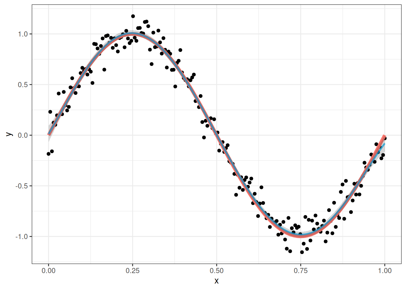
This is pretty close to perfect! So it seems like a fifth degree polynomial is a better choice than a third degree polynomial. The fit is so good that the confidence bands actually do a very good job at capturing the true relationship.
But why stop there? Maybe it is always better to increase the degree of the polynomial! Let’s try using a 150th degree polynomial for comparison:
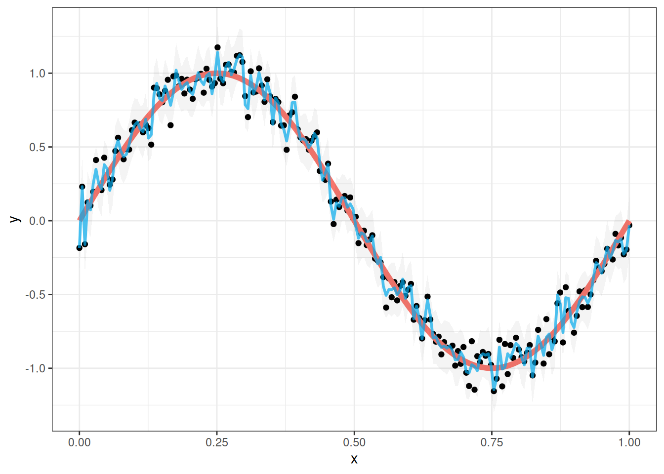
This no longer seems very good. The blue line above (which is the fit of the model to the data) is much less smooth than it should be. It zig-zags all over the place trying to fit each of the data points as well as possible. Additionally, the confidence bands around the sine curve are now much wider than they were with the 5th degree polynomial. What is going on here?
13.2 Overfitting
What we observed with the sine curve illustrates a fundamental concept in statistical modeling called overfitting. Overfitting occurs when a model learns to fit the noise in our data rather than the underlying relationship. Our 150th degree polynomial was clearly overfitting - it was trying so hard to fit each individual data point that it lost sight of the smooth, sinusoidal pattern that actually generated the data.
13.2.1 An Analogy: Studying for a Test
We can understand overfitting by considering how students prepare for exams using practice tests. Suppose we have a practice test with 25 questions about linear regression, and that the actual test also has 25 questions. Consider the following two strategies:
- A student might study the general concepts on the practice test and hope to do well based on the actual test.
- The student might memorize the answers to the practice test (e.g., A, B, A, C, A, B, B, …) and then answer those on the actual test.
What is going on with overfitting is similar to the second strategy: if we memorize the sequence of answers, we will do very well on the practice test. But we aren’t actually learning anything if we do this! And because the actual test won’t have the same sequence of answers as the practice test, we will end up doing poorly.
13.2.2 Overfitting and the Bias-Variance Tradeoff
Overfitting is typically understood through the bias-variance tradeoff. As mentioned many times throughout this course: the linearity assumption almost never holds exactly! Rather, what we really want is for the model to be “good enough” that we can behave as though the linearity assumption is correct without it affecting our conclusions.
In the case of the sine curve, neither the 5th degree nor the 150th degree polynomials are correct. The function \(\sin(x)\) can be expressed as
\[ \sin(x) = x - \frac{x^3}{3!} + \frac{x^5}{5!} - \frac{x^7}{7!} + \cdots \]
i.e., \(\sin(x)\) is a polynomial with an infinite degree. In fitting our polynomial approximations, we are observing the following:
- Our third degree fit is highly biased. No matter how much data we collect, a cubic polynomial will never adequately capture a sine curve - the model is fundamentally misspecified. The confidence band we see for the curve is very narrow, indicating high precision (low variance), but it misses the curve in many places (high bias).
- The 5th degree polynomial substantially reduces this bias; it is “just right”. The fitted curve tracks the true sine function more closely, and the 95% confidence bands generally contain the true curve and are still reasonably narrow. While still not perfect (recall that sine is an infinite-degree polynomial), the approximation is much better.
- The 150th degree polynomial, on the other hand, exhibits extremely high variance. While it has very low bias (in principle a 150th degree polynomial can model a sine curve very well), it is highly sensitive to the noise in our data. Each observation exerts significant influence on the fit, causing the curve to oscillate wildly between data points. We also see very wide confidence bands (indicating high variance) which nevertheless do contain the sine curve (suggesting low bias).
Correcting for overfitting is about properly calibrating between the bias (accuracy) and the variance (precision) of the model. The tradeoff is that if we want our models to be less biased we will typically need to make the models less precise. We can see this in the confidence intervals around our 150th degree polynomial, as not only did the estimate zig-zag but the width of the confidence intervals was also much wider than the other choices.
13.2.3 The Problem With \(R^2\)
Throughout this course, we have used \(R^2\) as a tool for measuring how well our regression models fit the data. We have typically interpreted \(R^2\) as the proportion of the variance in the dependent variable that can be accounted for by the variability in the independent variables. You might be wondering at this point:
Why do we need to think about overfitting? We already have \(R^2\) as a measure of how well the model fits. Why not just use that to decide which model is best?
A fundamental issue with \(R^2\) is that it always increases when we add more variables to the model. To see this, recall that
\[ R^2 = 1 - \frac{\text{SSE}}{\text{SST}} = 1 - \frac{\sum_i (Y_i - \widehat Y_i)^2}{\sum_i (Y_i - \bar Y)^2}. \]
If we add a variable to the model, the only part of the above expression that changes is \(\text{SSE}\); specifically, we know from the definition of least squares that the SSE of a bigger model is always smaller than the SSE of a smaller model. Consequently, adding variables can only decrease SSE and hence increase \(R^2\).
It follows that, as a measure of the quality of our model fit, \(R^2\) does not account for overfitting. If we include enough (possibly irrelevant) independent variables, eventually the \(R^2\) will climb all the way to \(1\)! To demonstrate this, it turns out that:
- The 5th degree polynomial has an \(R^2\) of about 98.1%
- The 150th degree polynomial has an \(R^2\) of about 99.5%
Even though the fit of the 150th degree polynomial is clearly worse visually than the 5th degree polynomial, if we go just by \(R^2\) we will end up using the overfit model instead!
The Main Point
The fact that \(R^2\) only increases when new variables are added means that it cannot be used by itself to select between models of different sizes: it will always favor the larger model, even when the smaller model might actually be better for prediction.
This problem with \(R^2\) is particularly acute when the number of predictors \(P\) approaches the sample size \(N\). In the extreme case where \(P = N\), we will always get \(R^2 = 1\), even if all of the predictors are totally irrelevant to the outcome! This is because with enough independent variables, we can always find a hyperplane that perfectly matches our data points, even if our independent variables have nothing to do with the dependent variable.
13.3 Sample Splitting
One of the most intuitive ways to deal with overfitting is through sample splitting. The core idea is simple: we divide our dataset into two (or more) pieces, use one piece to fit our model, and use the other piece to evaluate how well the model actually works. This approach is directly analogous to our idea of giving our model a “practice test” (which is referred to as the training data) and then evaluating the model on an “actual test” (which is referred to as the testing data). In the case of our 150th degree polynomial, we expect to do very well on the training data, but perform poorly on the testing data.
13.3.1 Train-Test Splitting
The most basic form of sample splitting is called train-test splitting. We randomly divide our data into two pieces: a training set that we use to fit our model and a testing set that we use to evaluate the model’s performance.
The picture you should have in mind when you think about train-test splitting is something like this:
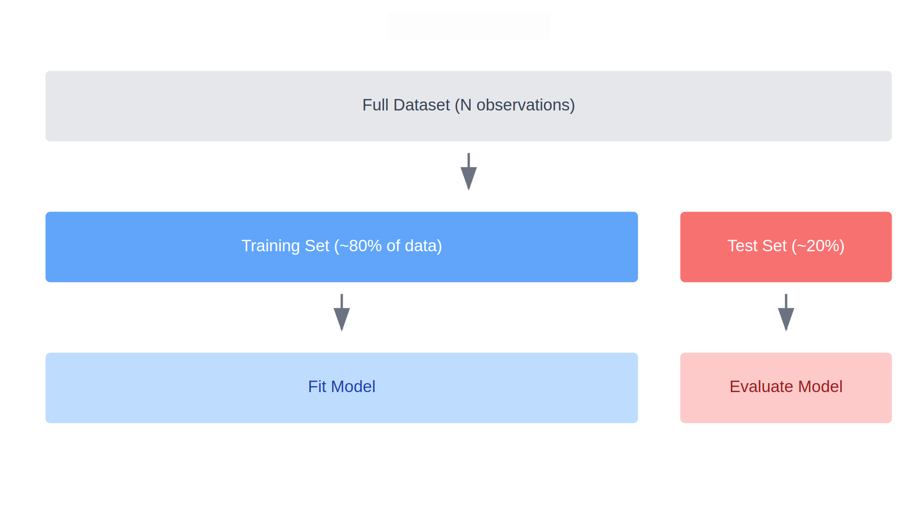
In this case, we are using 80% of the data for the training set and 20% for the testing set; this is reasonably standard as a splitting percent, but depending on the situation you might want different proportions.
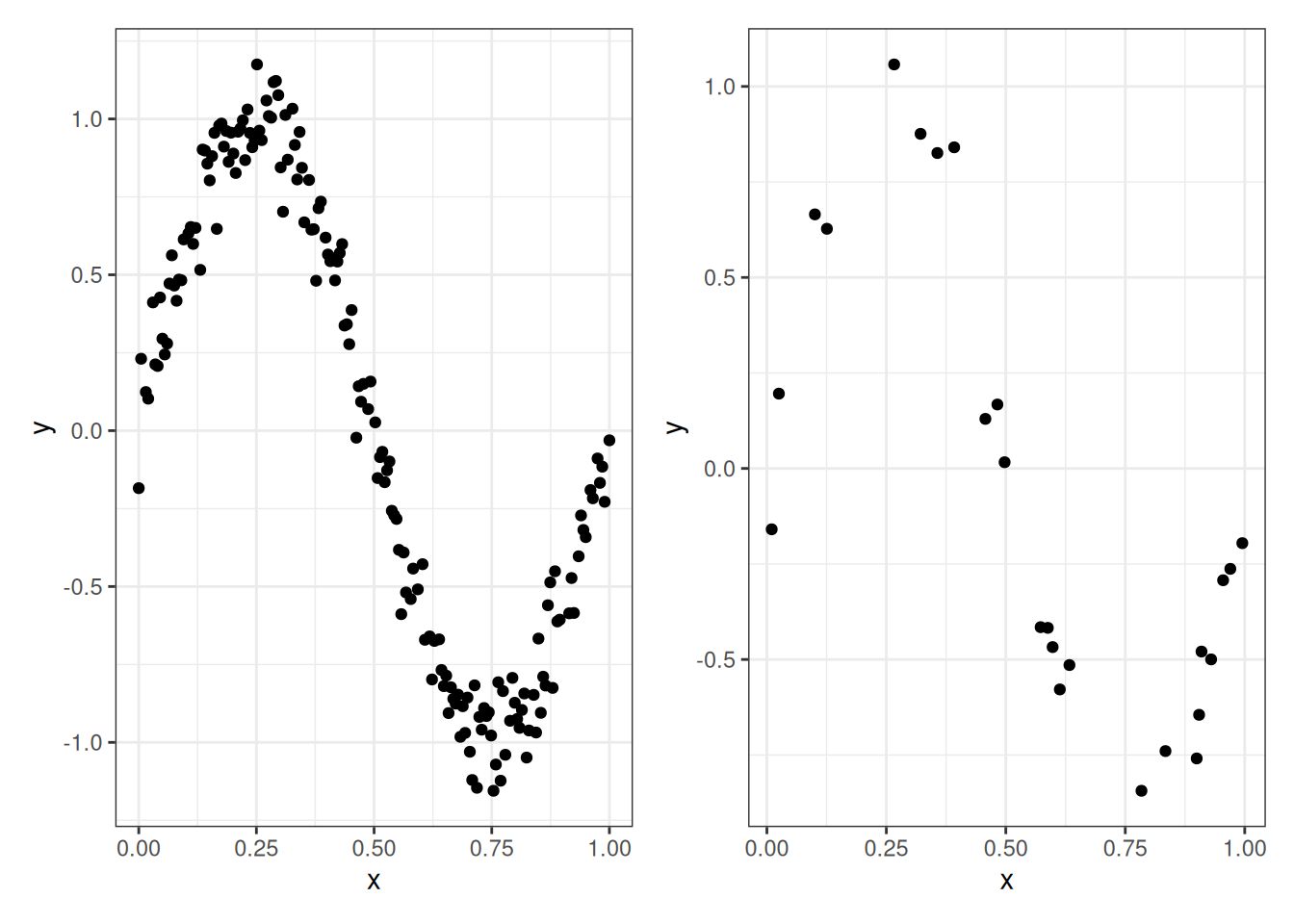
Let’s illustrate this on our sine curve example. Below we display a training set of 175 points (left) and a testing set of 25 points (right):
Next, we’ll fit the fifth-degree polynomial and 150th degree polynomial regressions to the training data and plot the results on the testing data:
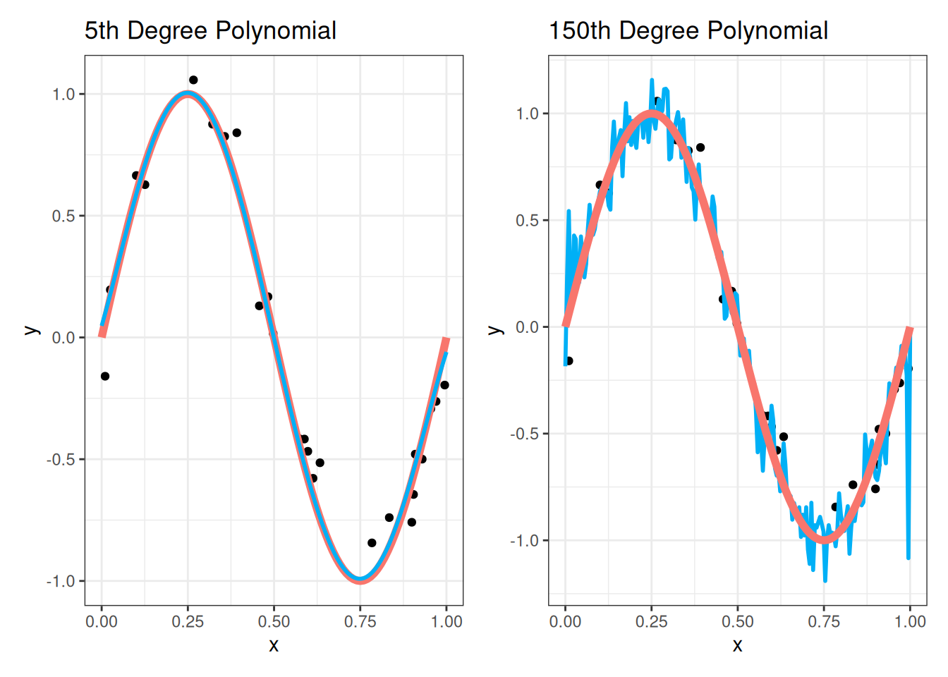
We see visually that the 5th degree polynomial fits the testing data much better than the 150th degree polynomial. Because the 150th degree polynomial overfits the training data, it does not generalize well to the testing data, and its zig-zagging behavior does not match the testing data points!
13.3.2 Evaluating Performance Using Train-Test Splits
To be a bit more precise, we can measure the performance of the different methods on the testing set using the mean squared error on the testing set. This is given by
\[ \text{MSE}_{\text{test}} = \frac{1}{N_{\text{test}}} \sum_i (Y_{i, \text{test}} - \widehat Y_{i, \text{test}})^2 \]
where:
- \(N_{\text{test}}\) is the number of observations in the testing set (25 in our case);
- \(Y_{i, \text{test}}\) denotes the observations \(i = 1,\ldots, N_{\text{test}}\) that are in the testing set;
- \(\widehat Y_{i, \text{test}}\) denotes the prediction of \(Y_{i, \text{test}}\) that we get when we use the model fit only to the training set.
For our sine curve example, it turns out that:
- \(\text{MSE}_{\text{test}}\) for the 5th degree polynomial is 0.013.
- \(\text{MSE}_{\text{test}}\) for the 150th degree polynomial is 0.067.
This validates our visual intuition that the 5th degree polynomial is better.
To see the effect of overfitting, we might incorrectly evaluate the model’s performance on the training set instead of the testing set. If we do this, we would instead get a mean squared error of 0.0094 for the 5th degree polynomial and 0.0016 for the 150th degree polynomial. The result for the 150th degree polynomial is highly misleading, as the MSE on the training data is over 40 times smaller than the MSE on the testing data.
One limitation of train-test splitting is that it can be sensitive to how we divide the data into training and testing sets. Usually this is done by assigning observations in the data randomly. If we were to randomly split the data a different way, we would get different results. Additionally, each observation is either in the training set or the testing set, so the individual observations are not treated equally. This leads us to cross-validation methods, which use multiple train-test splits to get more reliable estimates of model performance.
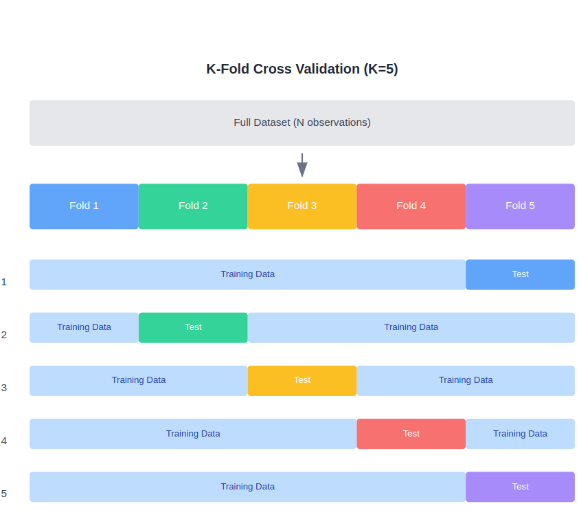
13.3.3 K-Fold Cross-Validation
K-fold cross-validation extends the train-test splitting idea by dividing the data into \(K\) roughly equal-sized pieces. We then fit our model K times, each time using a different fold as the testing set and the remaining K-1 folds as the training set. The picture you should have in mind with \(K\)-fold cross-validation is something like this:
Compared to using a single train-test split, \(K\)-fold cross-validation has the following benefits:
More stable evaluation: By using multiple train-test splits, we reduce the variance in our performance estimates that comes from the randomness of the split. A single train-test split might give us an unusually good or bad estimate just by chance.
More efficient use of data: Each observation gets to be in the test set exactly once and in the training set \(K-1\) times. In contrast, with a single train-test split, a significant portion of data is reserved for testing and not used in training.
More accurate performance estimation: The final cross-validation estimate is an average over \(K\) different test sets, making it more reliable than an estimate based on a single test set. This is particularly important when we have a small dataset where any single test set might not be representative of the population.
The main disadvantage of K-fold cross-validation is its computational cost: we need to fit the model \(K\) times rather than just once. However, for linear regression, this cost is usually quite modest, and the benefits typically outweigh this drawback.
While \(K\)-fold cross-validation is very useful, we actually will not be using it in this class; I mention it only to make you aware of its existence, because it is extremely useful in machine learning contexts, and to motivate the tool that we actually will use (leave-one-out cross-validation).
K-Fold Cross-Validation in R
If you really want to use \(K\)-fold cross-validation for whatever reason (for example, if you are using a method other than linear regression) then the caret package in R is the best option. Performing K-fold cross-validation with caret is discussed in Chapter 5 of this book.
13.3.4 Leave One Out (LOO) Cross-Validation
Leave-one-out cross-validation (LOOCV) is the special case of \(K\)-fold cross-validation where \(K\) equals the sample size \(N\). That is, we create \(N\) different training sets, each omitting a single observation, fit our model on each training set, and then evaluate how well we predict the left-out observation. This is an extreme version of \(K\)-fold cross-validation: every observation serves as the testing set once, while being part of the training set in all other iterations.
The immediate problem with LOOCV is that it appears to require fitting \(N\) separate linear regressions. This might not be a big deal with modern computing when \(N\) is small (for the sine curve example, your computer can fit \(200\) separate polynomial regressions extremely quickly), but things actually become quite problematic when \(N\) is very large. Remarkably, for linear regression, there’s actually a shortcut that allows us to compute the leave-one-out (LOO) fitted values without having to refit the model \(N\) times. If we let \(\widehat Y_{i,-i}\) denote the prediction for the \(i^{\text{th}}\) observation when we fit the model without that observation, then
\[ \widehat Y_{i,-i} = Y_i - \frac{e_i}{1 - h_{i}} \]
where \(e_i\) is the \(i^{\text{th}}\) residual from the full model fit and \(h_i\) is the leverage that we defined in Chapter 10.
With the LOO predictions, we can assess our model’s accuracy using the predicted residual error sum of squares (PRESS) statistic
\[ \text{PRESS} = \sum_i (Y_i - \widehat Y_{i,-i})^2. \]
PRESS is basically the same thing as SSE, except that rather than using \(\widehat Y_i\) you use \(\widehat Y_{i,-i}\), and can be interpreted in basically in the same way. Generally, we prefer models that have a small value of PRESS. The PRESS statistic can be computed using the press function in the package DAAG. Let’s compute PRESS for many different choices of the degree of the polynomial for the sine data:
## Note: there are less verbose ways to do this using, e.g., a loop or an apply
## function

## Install DAAG if you don't have it
library(DAAG)

poly_lm_3 <- lm(y ~ poly(x,3), data = my_sin_data)
poly_lm_4 <- lm(y ~ poly(x,4), data = my_sin_data)
poly_lm_5 <- lm(y ~ poly(x,5), data = my_sin_data)
poly_lm_6 <- lm(y ~ poly(x,6), data = my_sin_data)
poly_lm_7 <- lm(y ~ poly(x,7), data = my_sin_data)
poly_lm_8 <- lm(y ~ poly(x,8), data = my_sin_data)
poly_lm_9 <- lm(y ~ poly(x,9), data = my_sin_data)
poly_lm_10 <- lm(y ~ poly(x,10), data = my_sin_data)

press_df <- data.frame(degree = 3:10,
           PRESS = c(press(poly_lm_3),
                     press(poly_lm_4),
                     press(poly_lm_5),
                     press(poly_lm_6),
                     press(poly_lm_7),
                     press(poly_lm_8),
                     press(poly_lm_9),
                     press(poly_lm_10)))

plot(press_df$degree, press_df$PRESS, xlab = "Degree", ylab = "PRESS")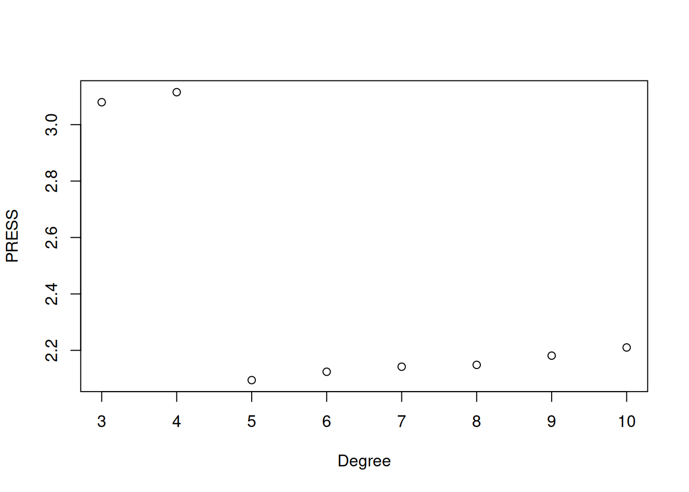
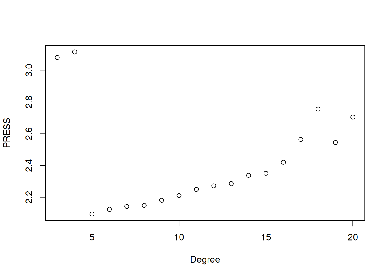
The plot shows how the PRESS statistic changes with polynomial degree. We see that it decreases sharply up through degree 5, suggesting that adding terms up to this point substantially improves predictive performance. After degree 5, the PRESS slowly increases, indicating that additional polynomial terms are leading to overfitting. This matches our earlier visual assessment, that a 5th degree polynomial provided a good balance between model complexity and predictive accuracy. If we carry this out to degree 20 we see clear signs of overfitting, with the performance deteriorating significantly as we increase the degree:
Limitations
The main downside to LOOCV is that it only really works efficiently for linear regression because, for other models, we cannot derive a shortcut formula and thus have to fit \(N\) separate models.
13.3.5 Getting the LOO Predictions in R
As far as I know, there is no built-in function that returns the LOO predictions. Instead, we can implement this on our own by defining our own function:
loo_predictions <- function(fit) {
  e <- residuals(fit)
  h <- hatvalues(fit)
  Y <- fitted(fit) + e
  return(Y - e / (1 - h))
}
Warning
You have to run this code in your script if you want to use this function. If you don’t do this then R will give an error saying that the function is not found.
The above function is based on the formula for the LOO predictions we gave earlier. After creating this function, we can get the LOO predictions by plugging the model fit into the function. For example, we can get the LOO predictions for the fifth degree polynomial by running
poly_lm_5 <- lm(y ~ poly(x, 5), data = my_sin_data)
loo_fitted_5 <- loo_predictions(poly_lm_5)
After making these, we can compare the LOO fitted values to the data:
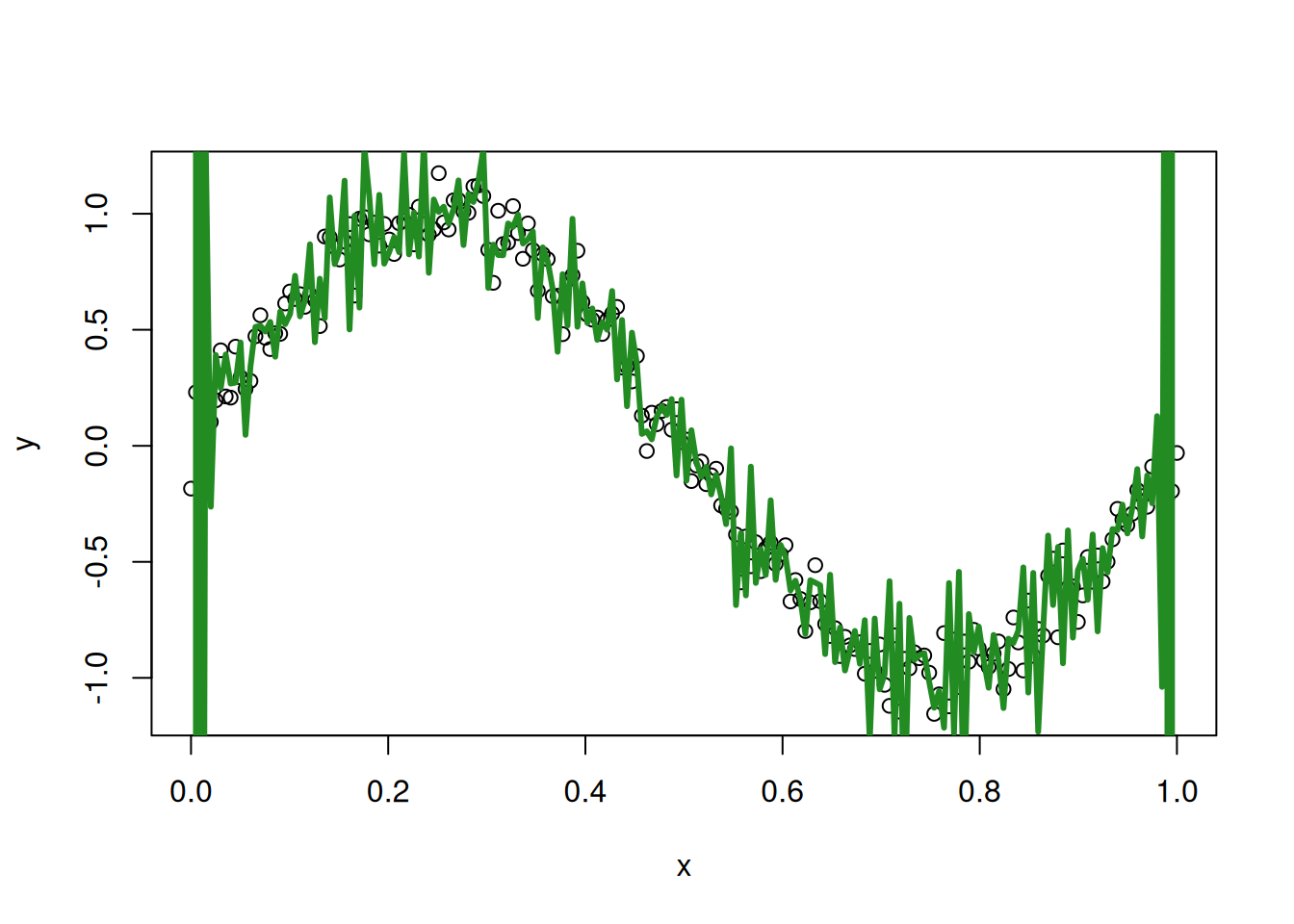
plot(my_sin_data$x, my_sin_data$y, xlab = "x", ylab = "y")
lines(my_sin_data$x, loo_fitted_5, col = 'forestgreen', lwd = 3)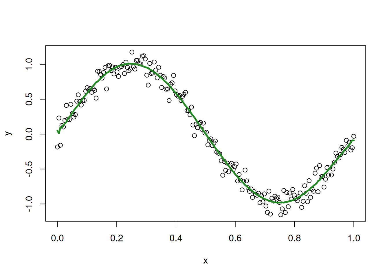
The LOO fitted values are a bit more jittery than the original fitted values, but they still seem to track the sine curve reasonably well. For comparison, this is what we get for a 20th degree polynomial:
poly_lm_20 <- lm(y ~ poly(x, 20), data = my_sin_data)
loo_fitted_20 <- loo_predictions(poly_lm_20)
plot(my_sin_data$x, my_sin_data$y, xlab = "x", ylab = "y")
lines(my_sin_data$x, loo_fitted_20, col = 'forestgreen', lwd = 3)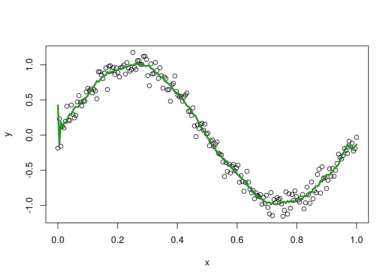
and our 150th degree polynomial:
Especially at the boundary, we see that things have completely broken down with our overfit 150th degree polynomial.
13.4 Penalized Goodness of Fit Measures
In this section we describe some commonly used alternatives to cross-validation and PRESS. These (mostly) correspond to taking one of the goodness-of-fit measures (like \(R^2\) or SSE) and tweaking it a little bit to account for possible overfitting. These tweaks known as penalties. Some of these we have also seen in the output of summary(), glance(), or anova(), so this provides a good opportunity to close the loop on what is available in these functions.
13.4.1 Adjusted \(R^2\)
Throughout the course we have been using multiple \(R^2\) as a measure of how much of the variability in the dependent variable can be captured by variability in the independent variables. While popular, \(R^2\) has a significant drawback: it always increases (or, at least, never decreases) when we add more independent variables into the model, even if they are truly unrelated to the outcome. This property can lead to overfitting if we try to use \(R^2\) to decide between two models.
To address this issue, it is sometimes recommended to use the adjusted \(R^2\) statistic, which adjusts \(R^2\) so that it no longer always increases when more variables are added to the model. The adjusted \(R^2\) is defined as:
\[ \text{Adjusted } R^2 = 1 - \frac{(1-R^2)(N-1)}{N-P-1}. \]
where, as usual, \(N\) is the number of observations and \(P\) is the number of coefficients (ignoring the intercept). The fact that adjusted \(R^2\) can potentially decrease when variables are added to the model makes it more suitable than regular \(R^2\) for comparing models of different sizes. To illustrate this, let’s take another look at the GPA dataset:
fygpa <- read.csv("https://raw.githubusercontent.com/theodds/SDS-348/master/satgpa.csv")
fygpa$sex <- ifelse(fygpa$sex == 1, "Male", "Female")
Now, let’s fit a regression model that includes
- all of the independent variables (high school GPA, sex, and SAT verbal/math scores) and
- all of the independent variables, plus an interaction between sex and SAT math score.
Below we fit the model:
fygpa_all <- lm(fy_gpa ~ hs_gpa + sex + sat_m + sat_v, data = fygpa)
fygpa_interact <- lm(fy_gpa ~ hs_gpa + sex + sat_m + sat_v + sex * sat_m,
                data = fygpa)
We then look at the results with summary():
summary(fygpa_all)
Call:
lm(formula = fy_gpa ~ hs_gpa + sex + sat_m + sat_v, data = fygpa)

Residuals:
    Min      1Q  Median      3Q     Max
-2.0601 -0.3478  0.0315  0.4106  1.7042

Coefficients:
             Estimate Std. Error t value Pr(>|t|)
(Intercept) -0.835161   0.148617  -5.620 2.49e-08 ***
hs_gpa       0.545008   0.039505  13.796  < 2e-16 ***
sexMale     -0.141837   0.040077  -3.539  0.00042 ***
sat_m        0.015513   0.002732   5.678 1.78e-08 ***
sat_v        0.016133   0.002635   6.123 1.32e-09 ***
---
Signif. codes:  0 '***' 0.001 '**' 0.01 '*' 0.05 '.' 0.1 ' ' 1

Residual standard error: 0.5908 on 995 degrees of freedom
Multiple R-squared:  0.3666,    Adjusted R-squared:  0.364
F-statistic: 144 on 4 and 995 DF, p-value: < 2.2e-16summary(fygpa_interact)
Call:
lm(formula = fy_gpa ~ hs_gpa + sex + sat_m + sat_v + sex * sat_m,
    data = fygpa)

Residuals:
     Min       1Q   Median       3Q      Max
-2.05350 -0.34605  0.03289  0.41173  1.72167

Coefficients:
               Estimate Std. Error t value Pr(>|t|)
(Intercept)   -0.787202   0.193277  -4.073 5.01e-05 ***
hs_gpa         0.544945   0.039522  13.788  < 2e-16 ***
sexMale       -0.238278   0.251543  -0.947    0.344
sat_m          0.014573   0.003651   3.991 7.07e-05 ***
sat_v          0.016161   0.002637   6.129 1.27e-09 ***
sexMale:sat_m  0.001779   0.004580   0.388    0.698
---
Signif. codes:  0 '***' 0.001 '**' 0.01 '*' 0.05 '.' 0.1 ' ' 1

Residual standard error: 0.591 on 994 degrees of freedom
Multiple R-squared:  0.3667,    Adjusted R-squared:  0.3635
F-statistic: 115.1 on 5 and 994 DF,  p-value: < 2.2e-16
Comparing these models strictly in terms of multiple \(R^2\), we see that the second model has a slightly higher \(R^2\) of 36.67% (versus 36.66%).
Adjusted \(R^2\) also appears in the output of the table here:
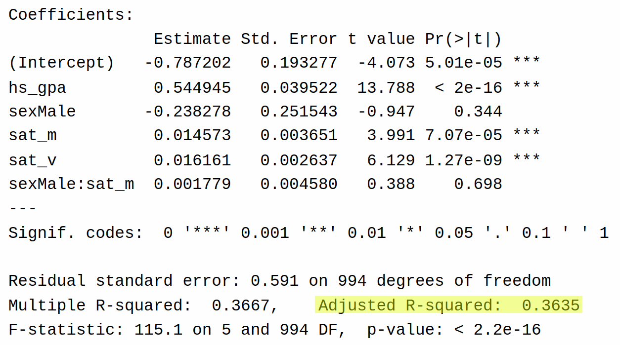
Comparing the adjusted \(R^2\) for the two models, we see that the model with the interaction has a lower adjusted \(R^2\) than the model without the interaction (36.35% versus 36.40%). So, at least in this case, adjusted \(R^2\) prefers the simpler model. This makes some intuitive sense as well based on the output of the coefficients: for the model with the interaction, we see that there is basically no evidence supporting the existence of the interaction between sex and sat_m (\(P\)-value of 0.698).
Adjusted \(R^2\) can also be used to decide on the degree of our polynomial on the sine example. Below I give a plot of adjusted \(R^2\) for different polynomial degrees:
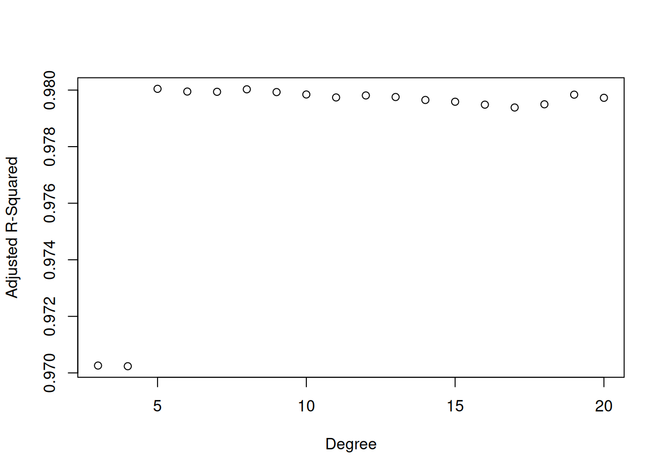
Adjusted \(R^2\) correctly picks out the degree \(5\) as being the best choice.
Don’t Use Adjusted \(R^2\)
In my experience, adjusted \(R^2\) - while certainly an improvement over \(R^2\) for model selection - tends not to be aggressive enough in combating overfitting. I mainly am covering adjusted \(R^2\) because it is common and appears in the output of summary() and glance(). Of the methods for dealing with overfitting that we will cover, I think adjusted \(R^2\) is the worst option. The LOO \(R^2\) discussed next is, in my experience, much better.
13.4.2 Leave One Out \(R^2\)
The adjusted \(R^2\) is an improvement over \(R^2\) for the purpose of model comparison, but it is still not ideal: the adjustment factor is not very intuitive, and arises from some hard-to-explain mathematics. It also turns out to be too lenient in that it tends to favor larger regression models than it is supposed to.
An alternative to adjusted \(R^2\) that I quite like is what I call the leave one out \(R^2\) (or LOO \(R^2\)). The idea is to modify the definition of \(R^2\) so that it uses the LOO fitted values \(\widehat Y_{i, -i}\) (i.e., the predicted value of \(Y_i\) when the \(i^{\text{th}}\) row of the dataset is removed) rather than the usual fitted values \(\widehat Y_i\). That is, rather than using the expression
\[ R^2 = \text{Correlation}(Y_i, \widehat Y_i)^2 \]
we might instead use
\[ R^2_{\text{loo}} = \text{Correlation}(Y_i, \widehat Y_{i,-i})^2 \]
where \(\text{Correlation}(Y_i, \widehat Y_i)\) denotes taking the usual correlation between the \((Y_1, \ldots, Y_N)\) and \((\widehat Y_1, \ldots, \widehat Y_N)\).
We can compute \(R^2_{\text{loo}}\) using the LOO trick for the polynomial data (3rd, 5th, and 150th degrees) as follows:
## Get LOO predictions for the 3rd, 5th, and 150th degree polynomials
loo_poly_3 <- loo_predictions(poly_lm_3)
loo_poly_5 <- loo_predictions(poly_lm_5)
loo_poly_150 <- loo_predictions(poly_lm_150)

## Get the LOO R-Squared
loo_data <- data.frame(
  degree = c(3, 5, 150),
  LOORSq = c(cor(loo_poly_3, my_sin_data$y)^2, cor(loo_poly_5, my_sin_data$y)^2,
             cor(loo_poly_150, my_sin_data$y)^2)
)

print(loo_data)
degree LOORSq
1 3 0.9692312720
2 5 0.9790729277
3 150 0.0002064385Of these options, the 5th degree polynomial is best, the 3rd degree polynomial is slightly worse, and the 150th degree polynomial is a catastrophe.
Different Definitions
The definition of \(R^2_{\text{loo}}\) I gave above is what I think the definition of this quantity “should” be. In reality, there have been a bunch of different attempts to define a leave-one-out version of \(R^2\), so if you look it up from a different source you might get a different definition that gives slightly different results. The approach I took was to make \(R^2_{\text{loo}}\) a squared correlation (and not think about making it a proportion of variability explained). Other approaches try to define it as a proportion of variability explained. I have never encountered a practical scenario where these different choices of \(R^2_{\text{loo}}\) lead to different results.
13.4.3 Akaike Information Criterion (AIC)
A limitation of adjusted \(R^2\) and LOO \(R^2\) is that they are, for the most part, limited to applications with numeric dependent variables, i.e., they are limited to applications with multiple linear regression.
A more general tool that can be used with many different types of models (some of which we will learn about towards the end of the course) is the Akaike Information Criterion or AIC. For the multiple linear regression model, the AIC is given by
\[ \text{AIC} = N \ln(\text{SSE} / N) + 2 P \]
There are also versions of AIC for other models we will look at towards the end of this course (which consider qualitative and count variables as the outcome). We can get AIC using the AIC function:
## Get the AIC for the 5th, 10th, and 150th degree polynomials
c(AIC(poly_lm_5, poly_lm_10, poly_lm_150))
$df
[1] 7 12 152
$AIC
[1] -344.8248 -338.0543 -341.0026In the case of AIC, lower is better. The model with the smallest AIC in this case is the 5th degree polynomial (-344.8 is smaller than -338.0 and -341.0).
(Optional) What is AIC Doing?
Admittedly, the formula for AIC is not really very intuitive. Essentially what AIC is trying to do is estimate an abstract “distance” from the estimated model to the true process that generated the data, and by selecting the AIC that is smallest we are trying to minimize this distance.
Given the level of the course, it is a bit difficult to be more precise than this. AIC was originally motivated by the field of information theory, which is beyond the scope of this course, and you can get more details from the Wikipedia page.
How AIC Deals With Overfitting
AIC is determined by two terms:
- The term \(N \ln (\text{SSE} / N)\), which is mainly determined by SSE.
- The term \(2P\), which counts the number of predictors.
The first term is small when SSE is small, so the first term encourages us to use models that fit the data well. If we just used the first term, we would always select the most complicated model, for the same reason that \(R^2\) always selects the most complicated model.
The second term penalizes models that include a lot of variables. The more variables we include, the bigger \(2P\) will be, which will prevent overfit models from having the smallest AIC.
The best model by AIC will therefore be the one that strikes the best compromise: we want to make SSE small, but to include a predictor we need to improve SSE by a non-trivial amount.
13.4.4 Bayesian Information Criterion (BIC)
The Bayesian Information Criterion (BIC) is another tool for model selection that, like AIC, penalizes models for having too many coefficients. For multiple linear regression, BIC is defined as
\[ \text{BIC} = N \ln(\text{SSE} / N) + (\ln N) P. \]
Like AIC, lower values of BIC indicate better models. The key difference between AIC and BIC is the size of the penalty term: while AIC includes a penalty of \(2P\), BIC’s penalty is \(P \ln(N)\). Since \(\ln(N) > 2\) whenever \(N > 7\), BIC imposes a larger penalty for model complexity than AIC does. Because of this, AIC will tend to select more complicated models than BIC.
To compute BIC we can again use the AIC function, but we need to specify a new argument k = log(N) where N is the number observations in the dataset:
## Get the BIC for the 5th, 10th, and 150th degree polynomials
c(AIC(poly_lm_5, poly_lm_10, poly_lm_150, k = log(nrow(my_sin_data))))
$df
[1] 7 12 152
$AIC
[1] -321.7366 -298.4745 160.3416In terms of the ordering of the models, the results here are the same as for AIC: the best model is the 5th degree polynomial (BIC = -321.7) followed by the 10th (BIC = -298.4) and finally the 150th (BIC = 160.3).
AIC Versus BIC
In practical terms, BIC selects smaller models than AIC. This is because BIC has a larger penalty term.
Which of the two is better? This depends quite a bit on what you actually are trying to achieve with your analysis:
If we want to select a model that will tend to produce the best predictions then it turns out that AIC will be better on average. It errs on the side of including too many variables rather than excluding important ones, and from a prediction perspective, it’s usually worse to omit a useful variable than to include a useless one.
If we want to select a model that is the “true” model, then BIC will do this provided that the sample size is very large. By comparison, AIC will sometimes select the “true” model, but will occasionally select models that are too large, even if the sample size is very large.
So I would tend to recommend AIC if our end goal is prediction, and BIC if our end goal is (trying) to identify the “true” linear regression that gave rise to the data.
A reasonable complaint about BIC is that, because things usually aren’t exactly linear to begin with, it is not possible to select the “true” model. One could therefore argue that BIC is not that useful, because it presumes something that we know is not true (i.e., that the “true model” is one of the models we have under consideration).
13.5 Automatic Model Selection
We now have at our disposal a variety of tools for evaluating the quality of linear regression models that use different numbers of predictors. The purpose of automatic model selection is to use one of these tools to automatically choose our final model for us.
To illustrate concepts, we’ll use the Boston housing dataset:
Boston <- MASS::Boston
head(Boston)
crim zn indus chas nox rm age dis rad tax ptratio black lstat
1 0.00632 18 2.31 0 0.538 6.575 65.2 4.0900 1 296 15.3 396.90 4.98
2 0.02731 0 7.07 0 0.469 6.421 78.9 4.9671 2 242 17.8 396.90 9.14
3 0.02729 0 7.07 0 0.469 7.185 61.1 4.9671 2 242 17.8 392.83 4.03
4 0.03237 0 2.18 0 0.458 6.998 45.8 6.0622 3 222 18.7 394.63 2.94
5 0.06905 0 2.18 0 0.458 7.147 54.2 6.0622 3 222 18.7 396.90 5.33
6 0.02985 0 2.18 0 0.458 6.430 58.7 6.0622 3 222 18.7 394.12 5.21
medv
1 24.0
2 21.6
3 34.7
4 33.4
5 36.2
6 28.7For the purposes of this section, our goal will be to find a good model for predicting the median home value in a census tract (medv) using the other variables in the dataset. Fitting a linear regression to all the variables gives
boston_lm <- lm(medv ~ crim + zn + indus + chas + nox + rm + age + dis + rad +
                  tax + ptratio + black + lstat, data = Boston)
summary(boston_lm)
Call:
lm(formula = medv ~ crim + zn + indus + chas + nox + rm + age +
    dis + rad + tax + ptratio + black + lstat, data = Boston)

Residuals:
    Min      1Q  Median      3Q     Max
-15.595  -2.730  -0.518   1.777  26.199

Coefficients:
              Estimate Std. Error t value Pr(>|t|)
(Intercept)  3.646e+01  5.103e+00   7.144 3.28e-12 ***
crim        -1.080e-01  3.286e-02  -3.287 0.001087 **
zn           4.642e-02  1.373e-02   3.382 0.000778 ***
indus        2.056e-02  6.150e-02   0.334 0.738288
chas         2.687e+00  8.616e-01   3.118 0.001925 **
nox         -1.777e+01  3.820e+00  -4.651 4.25e-06 ***
rm           3.810e+00  4.179e-01   9.116  < 2e-16 ***
age          6.922e-04  1.321e-02   0.052 0.958229
dis         -1.476e+00  1.995e-01  -7.398 6.01e-13 ***
rad          3.060e-01  6.635e-02   4.613 5.07e-06 ***
tax         -1.233e-02  3.760e-03  -3.280 0.001112 **
ptratio     -9.527e-01  1.308e-01  -7.283 1.31e-12 ***
black        9.312e-03  2.686e-03   3.467 0.000573 ***
lstat       -5.248e-01  5.072e-02 -10.347  < 2e-16 ***
---
Signif. codes:  0 '***' 0.001 '**' 0.01 '*' 0.05 '.' 0.1 ' ' 1

Residual standard error: 4.745 on 492 degrees of freedom
Multiple R-squared:  0.7406,    Adjusted R-squared:  0.7338
F-statistic: 108.1 on 13 and 492 DF,  p-value: < 2.2e-16
Just eyeballing this output, it looks like we might be able to get away with removing some of these variables. For example, the \(P\)-values for indus and age are looking a little large, so maybe they are not needed.
There are a few ways to go about doing this. One idea is to drop the variables with large \(P\)-values, but this typically is not the preferred way of proceeding. Instead, it is usually preferred to use one of the aforementioned criteria for model evaluation (LOO R-squared, PRESS, AIC, BIC, etc) to rank the models. In this section, we will list out some possibilities, starting from the most conceptually simple (All Subsets selection) and ending with the most complicated (Forward-Backward selection).
13.5.1 Why Do Automatic Model Selection?
Before jumping into the problem of automatic model selection, I think it is a good idea to reflect on why we are doing this in the first place. There are many reasons for engaging in model selection, and some of them are better than others.
A bad reason to do automatic model selection is laziness on the part of the analyst. There are lots of possible models one could fit to data, and so far we have adopted the attitude of “you need to think carefully about your problem and what questions you are actually trying to answer when deciding what your model should be.” When understanding the effect of (say)
noxonmedv, the interpretation of this effect depends on what other variables (lstat,ptratio, etc) are being held constant; different models actually answer different questions. People don’t like thinking through these issues because it is hard; better to offload the thinking to an algorithm to avoid having to think too hard.This is bad for at least two reasons. First, oftentimes the questions that you are interested in answering require controlling for certain variables, regardless of whether they appear to help predict the outcome. The second reason is that people who are interested in offloading their thinking to an algorithm will also tend to not control for the fact that they did model selection when performing inference. Section 13.6 discusses this issue in detail.
A good reason to do automatic model selection is to avoid overfitting when your goal is to build a predictive model. If our goal is to build a model that has good predictive accuracy, and we want to use an automatic procedure for building that model that is robust to overfitting, then doing automatic model selection makes sense. The catch here is that your goal should be just getting good predictions, rather than trying to do any hypothesis testing or building confidence intervals.
Another good reason to do automatic model selection is if the question you are asking itself is “which of these variables is associated with the outcome?” For example, if I think that there exist some small set of genes that predict occurrence of a disease, but I don’t know which of the genes it is, then I might use automatic model selection to identify a collection of candidate genes for a follow-up study.
I’m sure there are other reasons to do model selection that aren’t listed above. Unfortunately, I think usually people who do automatic selection are doing it for a bad reason. For now, we’ll just assume that we have a good reason for doing model selection.
13.5.2 All Subsets Selection
One approach to automatically selecting a model is just to try out every possible model, rank them all according to (say) AIC, and then choose the model with the smallest AIC. Switching gears slightly, for the GPA dataset there are a total of 16 possible models:
- A model including none of the variables
sex,sat_m,sat_v, orhs_gpa. - There are four models that include exactly one of the four variables.
- There are six models that include exactly two of the four variables: (
sex,sat_m), (sex,sat_v), (sex,hs_gpa), (sat_m,sat_v), (sat_m,hs_gpa), (sat_v,hs_gpa). - There are four models that exclude exactly one of the variables.
- Finally, there is one model that includes all variables.
So there is a finite list of 16 models we might want to use. The “All Subsets” approach simply selects the one that makes AIC/BIC/PRESS/etc. as small as possible. We could then just fit all 16 models, compute whatever criteria we want, and pick the best one.
For the Boston dataset, it turns out that there are 8192 possible models (assuming no interactions or non-linearity), so it is quite cumbersome to fit all of them by hand. Fortunately, the lmSubsets package in R will do this automatically:
## run install.packages("lmSubsets") to install the package
library(lmSubsets)

all_subsets <- lmSubsets(medv ~ crim + zn + indus + chas + nox + rm + age + dis +
                           rad + tax + ptratio + black + lstat,
                         data = Boston)
After doing the selection, we can print the results using summary():
summary(all_subsets)Call:
lmSubsets(formula = medv ~ crim + zn + indus + chas + nox + rm +
age + dis + rad + tax + ptratio + black + lstat, data = Boston)
Statistics:
SIZE BEST sigma R2 R2adj pval Cp AIC BIC
2 1 6.215760 0.5441463 0.5432418 < 2.22e-16 362.75295 3288.975 3301.655
3 1 5.540257 0.6385616 0.6371245 < 2.22e-16 185.64743 3173.542 3190.448
4 1 5.229396 0.6786242 0.6767036 < 2.22e-16 111.64889 3116.097 3137.230
5 1 5.138580 0.6903077 0.6878351 < 2.22e-16 91.48526 3099.359 3124.718
6 1 4.993865 0.7080893 0.7051702 < 2.22e-16 59.75364 3071.439 3101.024
7 1 4.932627 0.7157742 0.7123567 < 2.22e-16 47.17537 3059.939 3093.751
8 1 4.881782 0.7221614 0.7182560 < 2.22e-16 37.05889 3050.438 3088.477
9 1 4.847431 0.7266079 0.7222072 < 2.22e-16 30.62398 3044.275 3086.540
10 1 4.820596 0.7301704 0.7252743 < 2.22e-16 25.86592 3039.638 3086.130
11 1 4.779708 0.7352631 0.7299149 < 2.22e-16 18.20493 3031.997 3082.715
12 1 4.736234 0.7405823 0.7348058 < 2.22e-16 10.11455 3023.726 3078.671
13 1 4.740496 0.7406412 0.7343282 < 2.22e-16 12.00275 3025.611 3084.783
14 1 4.745298 0.7406427 0.7337897 < 2.22e-16 14.00000 3027.609 3091.007This returns for each possible model size the performance of the best model of that size in terms of \(R^2\), adjusted \(R^2\), AIC, and BIC, as well as some other criteria that we won’t discuss. This allows us to decide which criteria we want to use. Sadly, PRESS is not given.
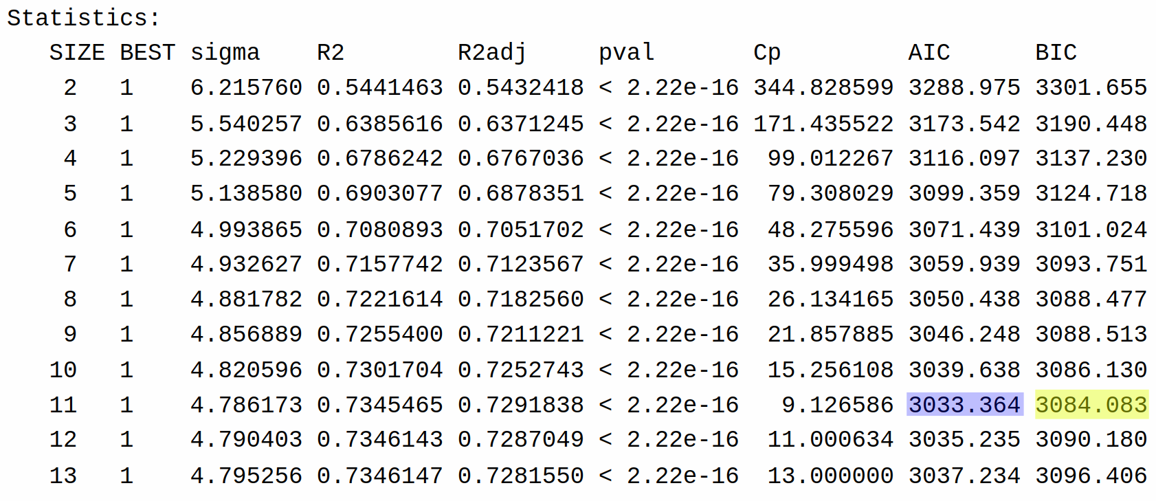
Whether we use AIC or BIC, we see that the best model is of size 11. We can see what variables are included in this model using the lmSelect() function. To select the best model using AIC we can run the following command:
lmSelect(all_subsets, penalty = "AIC")Call:
lmSelect(formula = medv ~ crim + zn + indus + chas + nox + rm +
age + dis + rad + tax + ptratio + black + lstat, data = Boston,
penalty = "AIC")
Criterion:
[best] = AIC
1st
3023.726
Subset:
best
+(Intercept) 1
crim 1
zn 1
indus
chas 1
nox 1
rm 1
age
dis 1
rad 1
tax 1
ptratio 1
black 1
lstat 1 Or, to select using BIC, we can run the command:
lmSelect(all_subsets, penalty = "BIC")Call:
lmSelect(formula = medv ~ crim + zn + indus + chas + nox + rm +
age + dis + rad + tax + ptratio + black + lstat, data = Boston,
penalty = "BIC")
Criterion:
[best] = BIC
1st
3078.671
Subset:
best
+(Intercept) 1
crim 1
zn 1
indus
chas 1
nox 1
rm 1
age
dis 1
rad 1
tax 1
ptratio 1
black 1
lstat 1 The entries under Subset tell us which variables are included; specifically, we include the variables with a 1 next to them, and discard the others. So, the final model excludes indus and age:
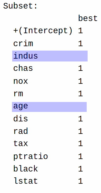
All other variables are included.
13.5.3 Backward Selection
A problem with the All Subsets approach is that it becomes impractical when there are many variables. Even with only four variables, using the All Subsets approach involves evaluating 16 possible models. In general, to find the best model according to All Subsets that features \(P\) different independent variables requires evaluating
\[ \text{number of possible models} = 2^P \]
linear regression models. So, for example, the Boston housing dataset has 13 predictors, which requires \(2^{13} = 8192\) possible models; still doable, but not fun. It’s not unusual to run into problems with 50 or more predictors, in which case you would need to evaluate \(2^{50} \approx 10^{15}\) models, which is not feasible with current technology. And for problems with (say) thousands of independent variables, All Subsets is completely out of the question. Now, computer scientists have worked hard on making All Subsets as practical as possible, and there are shortcuts that make it so that we do not have to actually fit all \(2^P\) models, so you can still do All Subsets with \(P = 50\) most of the time, but doing All Subsets is still impractical in many cases.
Instead of looking for the absolute best model according to AIC/BIC/PRESS, a common alternative is to perform backward selection.
I find backward selection easier to explain by example, so first let’s implement backward selection on the Boston housing dataset and then we will explain what the method is doing. Backward selection can be implemented using the step() function in R as follows:
Boston <- MASS::Boston
boston_lm <- lm(medv ~ crim + indus + chas + nox + rm + age + dis + rad + tax +
                  ptratio + black + lstat, data = Boston)
boston_step <- step(boston_lm, direction = "backward")
Start: AIC=1599.27
medv ~ crim + indus + chas + nox + rm + age + dis + rad + tax +
ptratio + black + lstat
Df Sum of Sq RSS AIC
- indus 1 0.01 11336 1597.3
- age 1 2.89 11339 1597.4
<none> 11336 1599.3
- tax 1 151.12 11487 1604.0
- crim 1 203.10 11539 1606.2
- chas 1 226.09 11562 1607.3
- black 1 276.73 11613 1609.5
- rad 1 412.32 11749 1615.3
- nox 1 513.49 11850 1619.7
- dis 1 979.28 12316 1639.2
- ptratio 1 1731.98 13068 1669.2
- rm 1 2145.96 13482 1685.0
- lstat 1 2334.43 13671 1692.0
Step: AIC=1597.27
medv ~ crim + chas + nox + rm + age + dis + rad + tax + ptratio +
black + lstat
Df Sum of Sq RSS AIC
- age 1 2.90 11339 1595.4
<none> 11336 1597.3
- tax 1 186.44 11523 1603.5
- crim 1 203.38 11540 1604.3
- chas 1 228.09 11564 1605.3
- black 1 277.20 11614 1607.5
- rad 1 446.21 11782 1614.8
- nox 1 555.29 11892 1619.5
- dis 1 1059.64 12396 1640.5
- ptratio 1 1786.88 13123 1669.3
- rm 1 2173.72 13510 1684.0
- lstat 1 2347.11 13683 1690.5
Step: AIC=1595.4
medv ~ crim + chas + nox + rm + dis + rad + tax + ptratio + black +
lstat
Df Sum of Sq RSS AIC
<none> 11339 1595.4
- tax 1 186.93 11526 1601.7
- crim 1 203.01 11542 1602.4
- chas 1 226.06 11565 1603.4
- black 1 274.75 11614 1605.5
- rad 1 453.52 11793 1613.2
- nox 1 630.01 11969 1620.8
- dis 1 1202.90 12542 1644.4
- ptratio 1 1834.82 13174 1669.3
- rm 1 2224.91 13564 1684.0
- lstat 1 2716.61 14056 1702.1The final model selected by backward selection removes the variables indus and age from the regression. Here is the logic that backward selection is using:
First, it fits the full model, and also the model with each of the individual predictors deleted, and computes the AIC. It lists the results of each of these single-term deletions in this table:
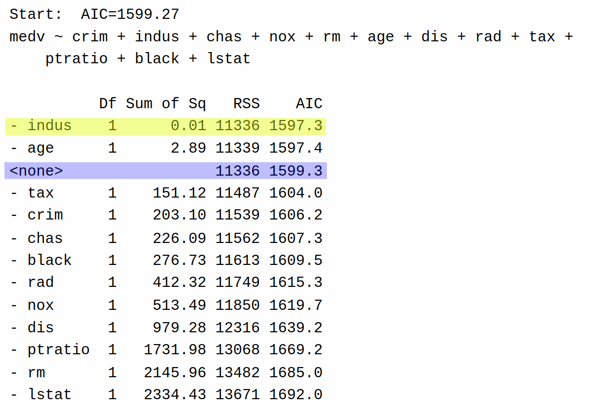
Highlighted yellow is the best decision according to AIC, while highlighted in blue is the “do nothing” move that returns the current model. Backward selection then decides to remove indus (AIC = 1597.3) from the model rather than keeping the full model (AIC = 1599.3) because doing so leads to a model with the lowest possible AIC (remember, lower AIC is better).
Having removed indus from the model, it next tries again, removing each of the other variables from the model to determine if it can reduce the AIC further:

Based on these results, backward selection decides that it can further reduce AIC by eliminating age from the model (AIC = 1595.4) rather than returning the model as-is with only indus removed (AIC = 1597.3). It then tries removing each of the variables one more time:
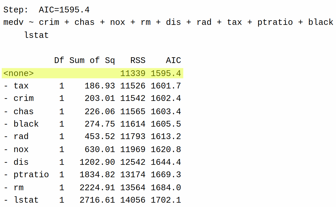
This time, however, the AIC cannot be decreased by removing another variable. Accordingly, backward selection stops at this step and returns the model with age and indus removed.
13.5.4 Forward Selection
Forward selection is the opposite of backward selection: rather than starting with a “big” model and removing variables, we start with a “small” model and consider adding variables. Again, I think it is easiest to understand via an example. We again use the function step(), but the usage is slightly different:
boston_intercept_only <- lm(medv ~ 1, data = Boston)
step(boston_intercept_only,
     scope = medv ~ crim + indus + chas + nox + rm + age + dis + rad + tax +
                  ptratio + black + lstat,
     direction = 'forward')
As input to step() we give a model that includes only the intercept, and also need to specify the biggest model we are willing to consider in the scope argument. After specifying these, and direction = "forward", a bunch of results will be printed off:
Start:  AIC=2246.51
medv ~ 1

          Df Sum of Sq   RSS    AIC
+ lstat    1   23243.9 19472 1851.0
+ rm       1   20654.4 22062 1914.2
+ ptratio  1   11014.3 31702 2097.6
+ indus    1    9995.2 32721 2113.6
+ tax      1    9377.3 33339 2123.1
+ nox      1    7800.1 34916 2146.5
+ crim     1    6440.8 36276 2165.8
+ rad      1    6221.1 36495 2168.9
+ age      1    6069.8 36647 2171.0
+ black    1    4749.9 37966 2188.9
+ dis      1    2668.2 40048 2215.9
+ chas     1    1312.1 41404 2232.7
<none>                 42716 2246.5

Step:  AIC=1851.01
medv ~ lstat

          Df Sum of Sq   RSS    AIC
+ rm       1    4033.1 15439 1735.6
+ ptratio  1    2670.1 16802 1778.4
+ chas     1     786.3 18686 1832.2
+ dis      1     772.4 18700 1832.5
+ age      1     304.3 19168 1845.0
+ tax      1     274.4 19198 1845.8
+ black    1     198.3 19274 1847.8
+ crim     1     146.9 19325 1849.2
+ indus    1      98.7 19374 1850.4
<none>                 19472 1851.0
+ rad      1      25.1 19447 1852.4
+ nox      1       4.8 19468 1852.9

Step:  AIC=1735.58
medv ~ lstat + rm

          Df Sum of Sq   RSS    AIC
+ ptratio  1   1711.32 13728 1678.1
+ chas     1    548.53 14891 1719.3
+ black    1    512.31 14927 1720.5
+ tax      1    425.16 15014 1723.5
+ dis      1    351.15 15088 1725.9
+ crim     1    311.42 15128 1727.3
+ rad      1    180.45 15259 1731.6
+ indus    1     61.09 15378 1735.6
<none>                 15439 1735.6
+ age      1     20.18 15419 1736.9
+ nox      1     14.90 15424 1737.1

Step:  AIC=1678.13
medv ~ lstat + rm + ptratio

        Df Sum of Sq   RSS    AIC
+ dis    1    499.08 13229 1661.4
+ black  1    389.68 13338 1665.6
+ chas   1    377.96 13350 1666.0
+ crim   1    122.52 13606 1675.6
+ age    1     66.24 13662 1677.7
<none>               13728 1678.1
+ tax    1     44.36 13684 1678.5
+ nox    1     24.81 13703 1679.2
+ rad    1      6.07 13722 1679.9
+ indus  1      0.83 13727 1680.1

Step:  AIC=1661.39
medv ~ lstat + rm + ptratio + dis

        Df Sum of Sq   RSS    AIC
+ nox    1    759.56 12469 1633.5
+ black  1    502.64 12726 1643.8
+ chas   1    267.43 12962 1653.1
+ indus  1    242.65 12986 1654.0
+ tax    1    240.34 12989 1654.1
+ crim   1    233.54 12995 1654.4
+ age    1     61.36 13168 1661.0
<none>               13229 1661.4
+ rad    1     22.40 13206 1662.5

Step:  AIC=1633.47
medv ~ lstat + rm + ptratio + dis + nox

        Df Sum of Sq   RSS    AIC
+ chas   1    328.27 12141 1622.0
+ black  1    311.83 12158 1622.7
+ crim   1    141.43 12328 1629.7
+ rad    1     53.48 12416 1633.3
<none>               12469 1633.5
+ indus  1     17.10 12452 1634.8
+ tax    1     10.50 12459 1635.0
+ age    1      0.25 12469 1635.5

Step:  AIC=1621.97
medv ~ lstat + rm + ptratio + dis + nox + chas

        Df Sum of Sq   RSS    AIC
+ black  1   272.837 11868 1612.5
+ crim   1   116.330 12025 1619.1
+ rad    1    58.556 12082 1621.5
<none>               12141 1622.0
+ indus  1    26.274 12115 1622.9
+ tax    1     4.187 12137 1623.8
+ age    1     2.331 12139 1623.9

Step:  AIC=1612.47
medv ~ lstat + rm + ptratio + dis + nox + chas + black

        Df Sum of Sq   RSS    AIC
+ rad    1   144.320 11724 1608.3
+ crim   1    55.633 11813 1612.1
<none>               11868 1612.5
+ indus  1    15.584 11853 1613.8
+ age    1     9.446 11859 1614.1
+ tax    1     2.703 11866 1614.4

Step:  AIC=1608.28
medv ~ lstat + rm + ptratio + dis + nox + chas + black + rad

        Df Sum of Sq   RSS    AIC
+ crim   1   197.793 11526 1601.7
+ tax    1   181.719 11542 1602.4
<none>               11724 1608.3
+ indus  1    27.983 11696 1609.1
+ age    1     2.981 11721 1610.2

Step:  AIC=1601.67
medv ~ lstat + rm + ptratio + dis + nox + chas + black + rad +
    crim

        Df Sum of Sq   RSS    AIC
+ tax    1   186.934 11339 1595.4
<none>               11526 1601.7
+ indus  1    35.701 11490 1602.1
+ age    1     3.386 11523 1603.5

Step:  AIC=1595.4
medv ~ lstat + rm + ptratio + dis + nox + chas + black + rad +
    crim + tax

        Df Sum of Sq   RSS    AIC
<none>               11339 1595.4
+ age    1   2.89621 11336 1597.3
+ indus  1   0.02095 11339 1597.4
Call:
lm(formula = medv ~ lstat + rm + ptratio + dis + nox + chas +
    black + rad + crim + tax, data = Boston)

Coefficients:
(Intercept)        lstat           rm      ptratio          dis          nox
  37.033189    -0.521889     4.003054    -1.096535    -1.177925   -18.632142
       chas        black          rad         crim          tax
   2.711816     0.009358     0.284364    -0.098193    -0.009548
Rather than starting with a “big” model and making it “smaller”, forward selection starts with a “small” model (using only the intercept) and making it “bigger”. So, the first step of forward selection gives the following table:
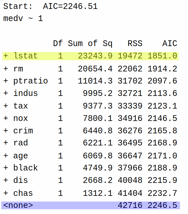
So at the first step of the forward selection algorithm, the algorithm decides it can reduce AIC the most by adding the variable lstat to the model (AIC = 1851) rather than keeping the model with only the intercept (AIC = 2246.5). It then repeats the process:
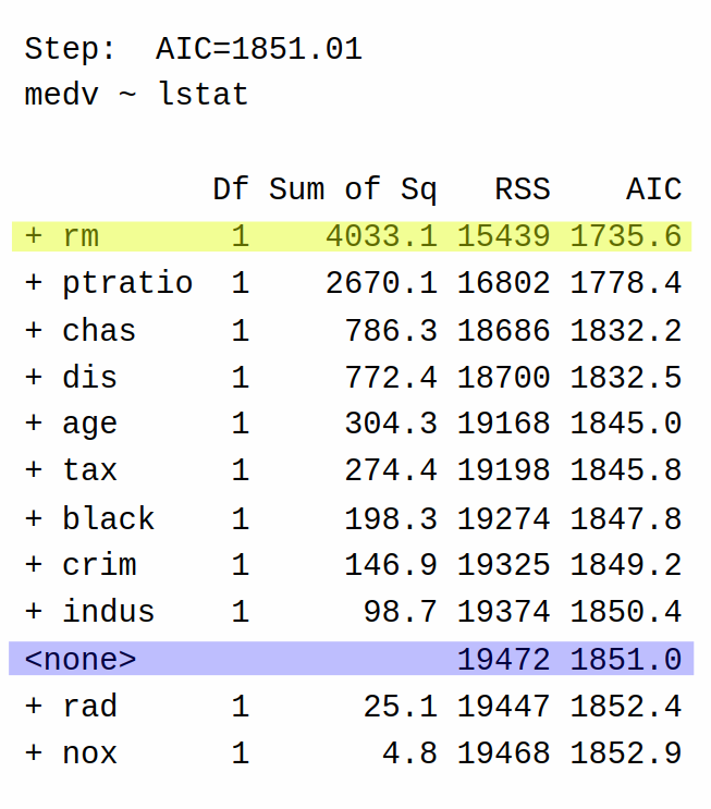
In the second step, the algorithm decides to add rm (AIC = 1735.6) rather than stopping at a model that only includes lstat (AIC = 1851.0).
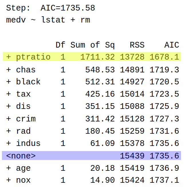
The third step adds ptratio. The process repeats many times until we reach the final step:
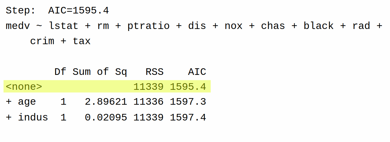
In the last step, the only options are to do nothing, add indus, or add age. This time, we cannot decrease AIC, and so the algorithm terminates and gives the same model as we got with backward selection.
Forward Selection and Backward Selection Don’t Always Agree
In this case, we got the same result with forward, backward, and all subsets selection. This isn’t always true! In practice, they all might give completely different models. If they do give different results, you can decide between them by using whichever approach gives the lower AIC.
13.5.5 Forward-Backward Selection
Forward-backward selection combines the ideas of forward and backward selection into a single procedure. The basic idea is that we consider
- deleting any of the currently-included variables from the model and
- adding any of the currently-excluded variables into the model (including those that we possibly deleted earlier).
This helps address a key limitation of pure forward selection: sometimes variables that were important early in the process become redundant after other variables are added.
To perform forward-backward selection, we use the argument direction = "both":
step(boston_lm, direction = "both")Start: AIC=1599.27
medv ~ crim + indus + chas + nox + rm + age + dis + rad + tax +
ptratio + black + lstat
Df Sum of Sq RSS AIC
- indus 1 0.01 11336 1597.3
- age 1 2.89 11339 1597.4
<none> 11336 1599.3
- tax 1 151.12 11487 1604.0
- crim 1 203.10 11539 1606.2
- chas 1 226.09 11562 1607.3
- black 1 276.73 11613 1609.5
- rad 1 412.32 11749 1615.3
- nox 1 513.49 11850 1619.7
- dis 1 979.28 12316 1639.2
- ptratio 1 1731.98 13068 1669.2
- rm 1 2145.96 13482 1685.0
- lstat 1 2334.43 13671 1692.0
Step: AIC=1597.27
medv ~ crim + chas + nox + rm + age + dis + rad + tax + ptratio +
black + lstat
Df Sum of Sq RSS AIC
- age 1 2.90 11339 1595.4
<none> 11336 1597.3
+ indus 1 0.01 11336 1599.3
- tax 1 186.44 11523 1603.5
- crim 1 203.38 11540 1604.3
- chas 1 228.09 11564 1605.3
- black 1 277.20 11614 1607.5
- rad 1 446.21 11782 1614.8
- nox 1 555.29 11892 1619.5
- dis 1 1059.64 12396 1640.5
- ptratio 1 1786.88 13123 1669.3
- rm 1 2173.72 13510 1684.0
- lstat 1 2347.11 13683 1690.5
Step: AIC=1595.4
medv ~ crim + chas + nox + rm + dis + rad + tax + ptratio + black +
lstat
Df Sum of Sq RSS AIC
<none> 11339 1595.4
+ age 1 2.90 11336 1597.3
+ indus 1 0.02 11339 1597.4
- tax 1 186.93 11526 1601.7
- crim 1 203.01 11542 1602.4
- chas 1 226.06 11565 1603.4
- black 1 274.75 11614 1605.5
- rad 1 453.52 11793 1613.2
- nox 1 630.01 11969 1620.8
- dis 1 1202.90 12542 1644.4
- ptratio 1 1834.82 13174 1669.3
- rm 1 2224.91 13564 1684.0
- lstat 1 2716.61 14056 1702.1
Call:
lm(formula = medv ~ crim + chas + nox + rm + dis + rad + tax +
    ptratio + black + lstat, data = Boston)

Coefficients:
(Intercept)         crim         chas          nox           rm          dis
  37.033189    -0.098193     2.711816   -18.632142     4.003054    -1.177925
        rad          tax      ptratio        black        lstat
   0.284364    -0.009548    -1.096535     0.009358    -0.521889
The process starts the same as backward selection, with indus being deleted. Then, in the second step, we see that we actually consider adding indus back in. In the third step, we also have steps corresponding to adding age back in or indus back in. The variables with a + next to them in the list correspond to adding the variable, while variables with a - next to them correspond to removing the variable.
One advantage of forward-backward selection over pure forward selection is that it can “correct mistakes” made early in the process. For example, suppose variable A is moderately useful by itself, but becomes completely redundant once we add variables B and C. Pure forward selection might add A early on and never remove it, while forward-backward selection has the opportunity to remove A after B and C enter the model.
13.5.6 Using BIC Instead
We have used AIC as our criterion for model selection, but we can just as easily use BIC or other criteria. Recall that BIC tends to select smaller models than AIC because it has a larger penalty for model complexity (\(\ln(N)\) versus 2 for each parameter). Let’s see how this plays out with the Boston housing data.
To use BIC instead of AIC with the step() function, we need to set k = log(n) where n is the sample size:
step(boston_lm, k = log(nrow(Boston)))Start: AIC=1654.21
medv ~ crim + indus + chas + nox + rm + age + dis + rad + tax +
ptratio + black + lstat
Df Sum of Sq RSS AIC
- indus 1 0.01 11336 1648.0
- age 1 2.89 11339 1648.1
<none> 11336 1654.2
- tax 1 151.12 11487 1654.7
- crim 1 203.10 11539 1657.0
- chas 1 226.09 11562 1658.0
- black 1 276.73 11613 1660.2
- rad 1 412.32 11749 1666.1
- nox 1 513.49 11850 1670.4
- dis 1 979.28 12316 1689.9
- ptratio 1 1731.98 13068 1719.9
- rm 1 2145.96 13482 1735.7
- lstat 1 2334.43 13671 1742.7
Step: AIC=1647.99
medv ~ crim + chas + nox + rm + age + dis + rad + tax + ptratio +
black + lstat
Df Sum of Sq RSS AIC
- age 1 2.90 11339 1641.9
<none> 11336 1648.0
- tax 1 186.44 11523 1650.0
- crim 1 203.38 11540 1650.8
- chas 1 228.09 11564 1651.8
- black 1 277.20 11614 1654.0
- rad 1 446.21 11782 1661.3
- nox 1 555.29 11892 1666.0
- dis 1 1059.64 12396 1687.0
- ptratio 1 1786.88 13123 1715.8
- rm 1 2173.72 13510 1730.5
- lstat 1 2347.11 13683 1737.0
Step: AIC=1641.89
medv ~ crim + chas + nox + rm + dis + rad + tax + ptratio + black +
lstat
Df Sum of Sq RSS AIC
<none> 11339 1641.9
- tax 1 186.93 11526 1643.9
- crim 1 203.01 11542 1644.6
- chas 1 226.06 11565 1645.7
- black 1 274.75 11614 1647.8
- rad 1 453.52 11793 1655.5
- nox 1 630.01 11969 1663.0
- dis 1 1202.90 12542 1686.7
- ptratio 1 1834.82 13174 1711.5
- rm 1 2224.91 13564 1726.3
- lstat 1 2716.61 14056 1744.3
Call:
lm(formula = medv ~ crim + chas + nox + rm + dis + rad + tax +
    ptratio + black + lstat, data = Boston)

Coefficients:
(Intercept)         crim         chas          nox           rm          dis
  37.033189    -0.098193     2.711816   -18.632142     4.003054    -1.177925
        rad          tax      ptratio        black        lstat
   0.284364    -0.009548    -1.096535     0.009358    -0.521889
Fortunately, in this case both AIC and BIC agree that the best model to use is the one that removes indus and age.
13.5.7 Which To Use?
We now have four methods for model selection: all subsets, backward, forward, and forward-backward. I’ll now attempt to give some insight, mostly from my own personal experience, regarding which methods will tend to work best.
- I usually prefer using AIC to BIC, as I am willing to tolerate some ‘irrelevant’ variables remaining after model selection. In most applications I work on, it’s a bigger mistake to exclude a variable that is actually needed than to include one that isn’t. However, this isn’t a universal truth.
- When possible, if I want to do automatic model selection, I will use All Subsets if I can. The main limiting factor to all subsets is that it cannot deal with moderate/large \(P\).
- When All Subsets fails I will do forward-backward selection, starting from a model that includes all of the candidate variables. It is rare that either forward selection on its own, or backward selection on its own, will do better than forward-backward.
- I will usually not do forward selection from an intercept-only model. The reason is just that it doesn’t seem to perform as well as backward or forward-backward. Some examples where forward selection fails, but backward and forward-backward selection succeed, are given in the exercises.
- The one case where we commonly do use forward selection is when there are a very large number of predictors; for example, if we have more predictors \(P\) than observations \(N\). You cannot even fit the model with all \(P\) predictors when \(P > N\), so a more natural starting point is the intercept-only model, using forward or forward-backward selection.
The following table summarizes things:
| Method | Advantages | Disadvantages |
|---|---|---|
| All Subsets | Finds the best model according to the criterion (and is the only approach that does) | Computationally infeasible for large \(P\) |
| Backward Selection | Simple to implement; starts with full model | Requires \(N > P\) |
| Forward Selection | Useful when \(P > N\); starts with minimal model | Can’t remove variables once added; some variables look promising initially end up not being useful, and we can’t remove them |
| Forward-Backward | Flexible; can add or remove variables | Computationally more intensive than forward/backward alone |
In practice, it’s often worth trying multiple methods and comparing their results. If they all select similar models, that increases our confidence in the selection. If they disagree substantially, that suggests we should be cautious about putting too much faith in any one model.
13.6 Post-Selection Inference
After using automatic model selection, one might hope to then proceed to do an analysis as usual: we might perform some hypothesis tests, construct some confidence intervals, and so forth. This turns out to be a mistake! Performing valid statistical inference after model selection turns out to be a subtle and challenging problem, because the standard inferential tools we’ve been using throughout the course are no longer valid after model selection. The problem of doing inference after performing model selection is known as post-selection inference.
To understand why post-selection inference is challenging, let’s consider what happens with the Boston housing data:
# Run stepwise selection
# The option trace = 0 makes it so that the output is not printed
boston_step <- step(boston_lm, direction = "both", trace = 0)

# Look at summary of selected model
summary(boston_step)
Call:
lm(formula = medv ~ crim + chas + nox + rm + dis + rad + tax +
    ptratio + black + lstat, data = Boston)

Residuals:
     Min       1Q   Median       3Q      Max
-15.9018  -2.8575  -0.7183   1.8759  26.7508

Coefficients:
              Estimate Std. Error t value Pr(>|t|)
(Intercept)  37.033189   5.116768   7.238 1.75e-12 ***
crim         -0.098193   0.032985  -2.977  0.00305 **
chas          2.711816   0.863245   3.141  0.00178 **
nox         -18.632142   3.552844  -5.244 2.33e-07 ***
rm            4.003054   0.406185   9.855  < 2e-16 ***
dis          -1.177925   0.162552  -7.246 1.65e-12 ***
rad           0.284364   0.063909   4.449 1.06e-05 ***
tax          -0.009548   0.003342  -2.857  0.00446 **
ptratio      -1.096535   0.122522  -8.950  < 2e-16 ***
black         0.009358   0.002702   3.463  0.00058 ***
lstat        -0.521889   0.047924 -10.890  < 2e-16 ***
---
Signif. codes:  0 '***' 0.001 '**' 0.01 '*' 0.05 '.' 0.1 ' ' 1

Residual standard error: 4.786 on 495 degrees of freedom
Multiple R-squared:  0.7345,    Adjusted R-squared:  0.7292
F-statistic:   137 on 10 and 495 DF,  p-value: < 2.2e-16
The \(P\)-values reported in this summary are misleading because they do not account for the fact that we performed model selection. The variables that remain in the model tend to have “significant” \(P\)-values partly because that’s what led to their selection in the first place!
To illustrate this issue more concretely, let’s do a simulation where we generate data with no true relationships. The following code generates a dependent variable \(Y\) along with \(P = 50\) completely irrelevant variables \(X\):
set.seed(999)
N <- 100
P <- 50

# Generate random predictors
X <- matrix(rnorm(N * P), N, P)
# Generate random noise for Y
y <- rnorm(N)

# Put into data frame
sim_data <- data.frame(y = y, X = X)
We then run model selection using AIC:
# Fit model and do selection
full_model <- lm(y ~ ., data = sim_data)
selected_model <- step(full_model, direction = "both", trace = 0)

# Look at summary
summary(selected_model)
Call:
lm(formula = y ~ X.3 + X.4 + X.5 + X.6 + X.8 + X.13 + X.14 +
    X.17 + X.18 + X.19 + X.20 + X.21 + X.22 + X.26 + X.28 + X.30 +
    X.31 + X.38 + X.40 + X.44 + X.47 + X.48 + X.49 + X.50, data = sim_data)

Residuals:
     Min       1Q   Median       3Q      Max
-1.36320 -0.46157  0.01414  0.48883  1.36103

Coefficients:
            Estimate Std. Error t value Pr(>|t|)
(Intercept)  0.07901    0.08317   0.950 0.345124
X.3         -0.19213    0.08082  -2.377 0.019990 *
X.4         -0.14296    0.08725  -1.639 0.105504
X.5         -0.13977    0.08181  -1.708 0.091695 .
X.6          0.21569    0.09490   2.273 0.025904 *
X.8         -0.24334    0.08976  -2.711 0.008313 **
X.13        -0.14813    0.09440  -1.569 0.120832
X.14         0.22077    0.08268   2.670 0.009295 **
X.17         0.27408    0.09163   2.991 0.003759 **
X.18         0.15765    0.08199   1.923 0.058304 .
X.19         0.24956    0.09427   2.647 0.009883 **
X.20        -0.28582    0.08198  -3.486 0.000822 ***
X.21         0.16582    0.08678   1.911 0.059850 .
X.22         0.14443    0.09345   1.545 0.126457
X.26        -0.18455    0.09856  -1.873 0.065031 .
X.28        -0.33662    0.08632  -3.900 0.000208 ***
X.30         0.25771    0.08348   3.087 0.002832 **
X.31         0.11696    0.08631   1.355 0.179476
X.38        -0.24596    0.09172  -2.682 0.009004 **
X.40         0.12782    0.08882   1.439 0.154296
X.44        -0.31665    0.08006  -3.955 0.000172 ***
X.47         0.24132    0.07766   3.107 0.002665 **
X.48        -0.30495    0.08554  -3.565 0.000637 ***
X.49        -0.27148    0.09342  -2.906 0.004811 **
X.50         0.26797    0.07724   3.469 0.000868 ***
---
Signif. codes:  0 '***' 0.001 '**' 0.01 '*' 0.05 '.' 0.1 ' ' 1

Residual standard error: 0.754 on 75 degrees of freedom
Multiple R-squared:  0.5966,    Adjusted R-squared:  0.4676
F-statistic: 4.623 on 24 and 75 DF,  p-value: 1.763e-07
Even though we generated \(Y\) completely independently of the \(X\) variables, we end up with “significant” \(P\)-values in the selected model! The overall \(F\)-test of model significance ends up having a highly significant \(P\)-value of \(\approx 1.7 \times 10^{-7}\). This happens because the selection process is deliberately seeking models where the selected variables can fit \(Y\) particularly well. In this case, there are \(2^{50} \approx 10^{15}\) possible models, and with so many models it is likely that some will appear significant purely by chance.
There are several approaches to doing valid inference after automatic model selection. The simplest solution is to just use data splitting, i.e.,
- Use one part of the data to perform the model selection.
- Use the other part of the data to do inference.
In the above setting, let’s pretend that we did the model selection on half the data, but that there is another batch of data we haven’t used yet, and see how the results differ:
# Generate test data
X_test <- matrix(rnorm(N * P), N, P)
y_test <- rnorm(N)
test_data <- data.frame(y = y_test, X = X_test)

# Fit the model that was selected
test_lm <- lm(y ~ X.3 + X.4 + X.5 + X.6 + X.8 + X.13 + X.14 +
    X.17 + X.18 + X.19 + X.20 + X.21 + X.22 + X.26 + X.28 + X.30 +
    X.31 + X.38 + X.40 + X.44 + X.47 + X.48 + X.49 + X.50,
    data = test_data)

summary(test_lm)
Call:
lm(formula = y ~ X.3 + X.4 + X.5 + X.6 + X.8 + X.13 + X.14 +
    X.17 + X.18 + X.19 + X.20 + X.21 + X.22 + X.26 + X.28 + X.30 +
    X.31 + X.38 + X.40 + X.44 + X.47 + X.48 + X.49 + X.50, data = test_data)

Residuals:
     Min       1Q   Median       3Q      Max
-2.28355 -0.67040  0.06157  0.64548  2.40246

Coefficients:
             Estimate Std. Error t value Pr(>|t|)
(Intercept) -0.000506   0.137247  -0.004    0.997
X.3         -0.102857   0.126692  -0.812    0.419
X.4          0.016437   0.134963   0.122    0.903
X.5          0.043208   0.126102   0.343    0.733
X.6          0.111925   0.121603   0.920    0.360
X.8         -0.003563   0.121154  -0.029    0.977
X.13        -0.019600   0.126732  -0.155    0.878
X.14        -0.172754   0.136840  -1.262    0.211
X.17         0.262309   0.140080   1.873    0.065 .
X.18        -0.113625   0.135302  -0.840    0.404
X.19        -0.103458   0.137366  -0.753    0.454
X.20         0.026566   0.133487   0.199    0.843
X.21         0.072630   0.160758   0.452    0.653
X.22        -0.002579   0.126432  -0.020    0.984
X.26         0.085346   0.137199   0.622    0.536
X.28         0.197375   0.136017   1.451    0.151
X.30         0.101184   0.125032   0.809    0.421
X.31        -0.106618   0.141888  -0.751    0.455
X.38        -0.025489   0.137679  -0.185    0.854
X.40         0.072565   0.116736   0.622    0.536
X.44        -0.067859   0.150413  -0.451    0.653
X.47        -0.026940   0.124922  -0.216    0.830
X.48         0.052608   0.156095   0.337    0.737
X.49         0.210896   0.146336   1.441    0.154
X.50        -0.003642   0.143347  -0.025    0.980
---
Signif. codes:  0 '***' 0.001 '**' 0.01 '*' 0.05 '.' 0.1 ' ' 1

Residual standard error: 1.172 on 75 degrees of freedom
Multiple R-squared:  0.1632,    Adjusted R-squared:  -0.1046
F-statistic: 0.6092 on 24 and 75 DF,  p-value: 0.9136
When we perform inference on the test data, we see that none of the predictors are actually statistically significant, which is what we would hope since none of them are actually relevant.
Warning
One thing that I find particularly striking in the above example is just how misleading the \(P\)-values we got after performing the automatic model selection were. Many of the \(P\)-values were so small that it would be reasonable to think that they are obviously relevant, and move on! The reality is that the \(P\)-values and confidence intervals you get after model selection can be comically misleading. To get valid statistical inference, doing something like data splitting is an absolute must.
The advantage of data splitting is that it’s simple, and the inference is valid. The disadvantage is that, with less data for model fitting and inference, our estimates become less precise, leading to wider confidence intervals and reduced ability to detect true effects.
13.7 Exercises
13.7.1 Exercise: MLB
The Hitters dataset contains Major League Baseball data from the 1986 and 1987 seasons. It is contained in the ISLR package, so make sure it is installed (install.packages("ISLR")). According to the documentation:
This dataset was taken from the StatLib library which is maintained at Carnegie Mellon University. This is part of the data that was used in the 1988 ASA Graphics Section Poster Session. The salary data were originally from Sports Illustrated, April 20, 1987. The 1986 and career statistics were obtained from The 1987 Baseball Encyclopedia Update published by Collier Books, Macmillan Publishing Company, New York.
We can then load the dataset by running
library(ISLR)
library(tidyverse)

# Load the data
data(Hitters)

# Remove missing data from the dataset
Hitters <- drop_na(Hitters)
and view it by running
head(Hitters) AtBat Hits HmRun Runs RBI Walks Years CAtBat CHits CHmRun
-Alan Ashby 315 81 7 24 38 39 14 3449 835 69
-Alvin Davis 479 130 18 66 72 76 3 1624 457 63
-Andre Dawson 496 141 20 65 78 37 11 5628 1575 225
-Andres Galarraga 321 87 10 39 42 30 2 396 101 12
-Alfredo Griffin 594 169 4 74 51 35 11 4408 1133 19
-Al Newman 185 37 1 23 8 21 2 214 42 1
CRuns CRBI CWalks League Division PutOuts Assists Errors
-Alan Ashby 321 414 375 N W 632 43 10
-Alvin Davis 224 266 263 A W 880 82 14
-Andre Dawson 828 838 354 N E 200 11 3
-Andres Galarraga 48 46 33 N E 805 40 4
-Alfredo Griffin 501 336 194 A W 282 421 25
-Al Newman 30 9 24 N E 76 127 7
Salary NewLeague
-Alan Ashby 475.0 N
-Alvin Davis 480.0 A
-Andre Dawson 500.0 N
-Andres Galarraga 91.5 N
-Alfredo Griffin 750.0 A
-Al Newman 70.0 AOur goal will be to predict the Salary of each player from their various attributes (see ?Hitters for a list).
Fit a model that predicts
Salaryusing all of the variables and store the result inhitters_1. Report the \(R^2\) and adjusted \(R^2\) for this model and interpret it in terms of the percentage of variability in salary explained by the variables.Now, fit a model that predicts
Salaryusing all pairwise interactions between the variables and store the result inhitters_2; this can be done by fitting a model with the formulaSalary ~ (.)^2. Report the \(R^2\) and adjusted \(R^2\) for this model; how does it compare with the model from part (a)?Plot
fitted(hitters_2)againstHitters$Salary. Does the model appear to be doing a good job? Explain.Now, plot
loo_predictions(hitters_2)againstHitters$Salary. Do you notice oddities in terms of the predicted salaries? Explain.Construct a model that includes some (but not all) of the interaction terms to make a new model
hitters_3that has a higher leave-one-out \(R^2\) thanhitters_1. Report the model that you settled on.
13.7.2 Exercise: Motorcycle
The dataset mcycle contains data from a simulated motorcycle accident used to test crash helmets. The variable times gives the time in milliseconds after the impact and accel gives the acceleration in terms of the force of gravity (g, i.e., 9.8 meters per second squared).
First, load the data:
mcycle <- MASS::mcyclePlot
times(on the x axis) againstaccel(on the y axis). How would you describe the relationship between time and acceleration? Is it linear?In terms of the plot you made above, can you think of any obvious ways (aside from non-linearity) that the usual regression modeling assumptions we have been making might fail?
We will consider polynomial regression models of the form \(Y_i = \beta_0 + \beta_1 \, X_i + \beta_2 \, X_i^2 + \cdots + \beta_B \, X_i^B + \epsilon_i\). This can be fit, for example, by running
lm(accel ~ poly(times, 2), data = mcycle)to fit a quadratic polynomial.Fit polynomials up-to degree 10 and report the leave-one-out R-Squared for each. Which degree fits best, and what is the leave-one-out R-squared associated with it?
Again plot
timeson the x axis andaccelon the y-axis, but add on the predicted accelerations (using, e.g.,predict) using thelinesfunction. Does the model look like it working well? Explain.
13.7.3 Exercise: When Things Break Down
This exercise concerns data taken from the article Mantel N (1970) Why stepdown procedures in variable selection? Technometrics, 12, 621–625.
The following loads the data:
mantel <- read.table("https://gattonweb.uky.edu/faculty/sheather/book/docs/datasets/Mantel.txt", header = TRUE)
head(mantel)
Y X1 X2 X3
1 5 1 1004 6.0
2 6 200 806 7.3
3 8 -50 1058 11.0
4 9 909 100 13.0
5 11 506 505 13.1The data were generated such that the full model
\[ Y_i = \beta_0 + \beta_1 \, X_{i1} + \beta_2 \, X_{i2} + \beta_3 \, X_{i3} + \epsilon_i \]
is valid. There are, in total, 8 possible models that we can consider:
- Intercept only.
- \(X_1\) only
- \(X_2\) only
- \(X_3\) only
- \(X_1\) and \(X_2\)
- \(X_1\) and \(X_3\)
- \(X_2\) and \(X_3\)
- All variables
Identify the optimal model or models based on adjusted \(R^2\), PRESS, AIC, and BIC from the approach based on all possible subsets. (You can do this by fitting eight separate models using
lmand computed these quantities on each of them.)Identify the optimal model or models based on AIC and BIC from the approach based on forward selection.
Carefully explain why different models are chosen in (a) and (b).
Decide which model you would recommend. Give detailed reasons to support your choice.
13.7.4 Exercise: Golf
An avid fan of the PGA tour with limited background in statistics has sought your help in answering one of the age-old questions in golf, namely, what is the relative importance of each different aspect of the game on average prize money in professional golf?
The following data are on the top 196 tour players in 2006:
pga_tour <- read_csv("https://gattonweb.uky.edu/faculty/sheather/book/docs/datasets/pgatour2006.csv")
head(pga_tour)
# A tibble: 6 × 12
Name TigerWoods PrizeMoney AveDrivingDistance DrivingAccuracy GIR
<chr> <dbl> <dbl> <dbl> <dbl> <dbl>
1 Aaron Baddeley 0 60661 288. 60.7 58.3
2 Adam Scott 0 262045 301. 62 69.1
3 Alex Aragon 0 3635 303. 51.1 59.1
4 Alex Cejka 0 17516 289. 66.4 67.7
5 Arjun Atwal 0 16683 288. 63.2 64.0
6 Arron Oberhols… 0 107294 285 62.5 69.3
# ℹ 6 more variables: PuttingAverage <dbl>, BirdieConversion <dbl>,
# SandSaves <dbl>, Scrambling <dbl>, BounceBack <dbl>, PuttsPerRound <dbl>It includes the following variables:
The outcome of interest
PrizeMoney.DrivingAccuracyis the percent of time a player is able to hit the fairway with his tee shot.GIR, Greens in Regulation is the percent of time a player was able to hit the green in regulation. A green is considered hit in regulation if any part of the ball is touching the putting surface and the number of strokes taken is two or less than par.PuttingAveragemeasures putting performance on those holes where the green is hit in regulation (GIR). By using greens hit in regulation the effects of chipping close and one putting are eliminated.BirdieConversionis the percent of time a player makes birdie or better after hitting the green in regulation.SandSavesis the percent of time a player was able to get “up and down” once in a greenside sand bunker.Scramblingis the percent of time that a player misses the green in regulation, but still makes par or better.PuttsPerRoundis the average total number of putts per round.
Fit a model regressing
PrizeMoneyon the variables listed above, as well as a model that uses the log-transformation ofPrizeMoney. After looking at diagnostic plots, which seems better?Using the
lmSubsetsfunction, Identify the optimal model or models based on AIC and BIC from the approach based on all possible subsets of the predictors. What models are best according to these criteria?Repeat part (b) using backward selection.
Identify the optimal model or models based on AIC and BIC from the approach based on forward selection.
Recommend a final model. Give detailed reasons to support your choice.
Interpret the regression coefficients of the final model. Is it necessary to be cautious about taking these results too literally?