12 Interaction Effects
For the multiple linear regression models we have considered so far, we’ve focused on understanding how the individual independent variables predict the dependent variable of interest by interpreting the \(\beta_j\)’s in the linear model
\[ Y_i = \beta_0 + \sum_j \beta_j \, X_{ij} + \epsilon_i. \]
In this model, each predictor contributes independently in predicting the outcome. This approach, while powerful, assumes that the effect of one variable remains constant regardless of the values of the other variables.
However, real-world phenomena are often more complex. For example, in practice we often find that medical treatments that are effective for men are more/less effective for women. This would be an example of an interaction effect: we have two independent variables in this example (sex and the medical treatment), and the effect of one of the variables depends on the other variable.
In this chapter, we’ll develop this idea more formally, and see how to build regression models that allow for interactions and how to interpret them.
12.1 Main Effects versus Interaction Effects
To illustrate the idea, suppose you are an education researcher investigating how study time affects test scores. Initially, we might expect a straightforward relationship: more study time leads to higher scores. However, it is often the case that students have different memory skills: what takes one student days of study time to learn might be mastered by other students in only a matter of hours. If this is the case, we might expect that the impact of study time is not uniform across all students.
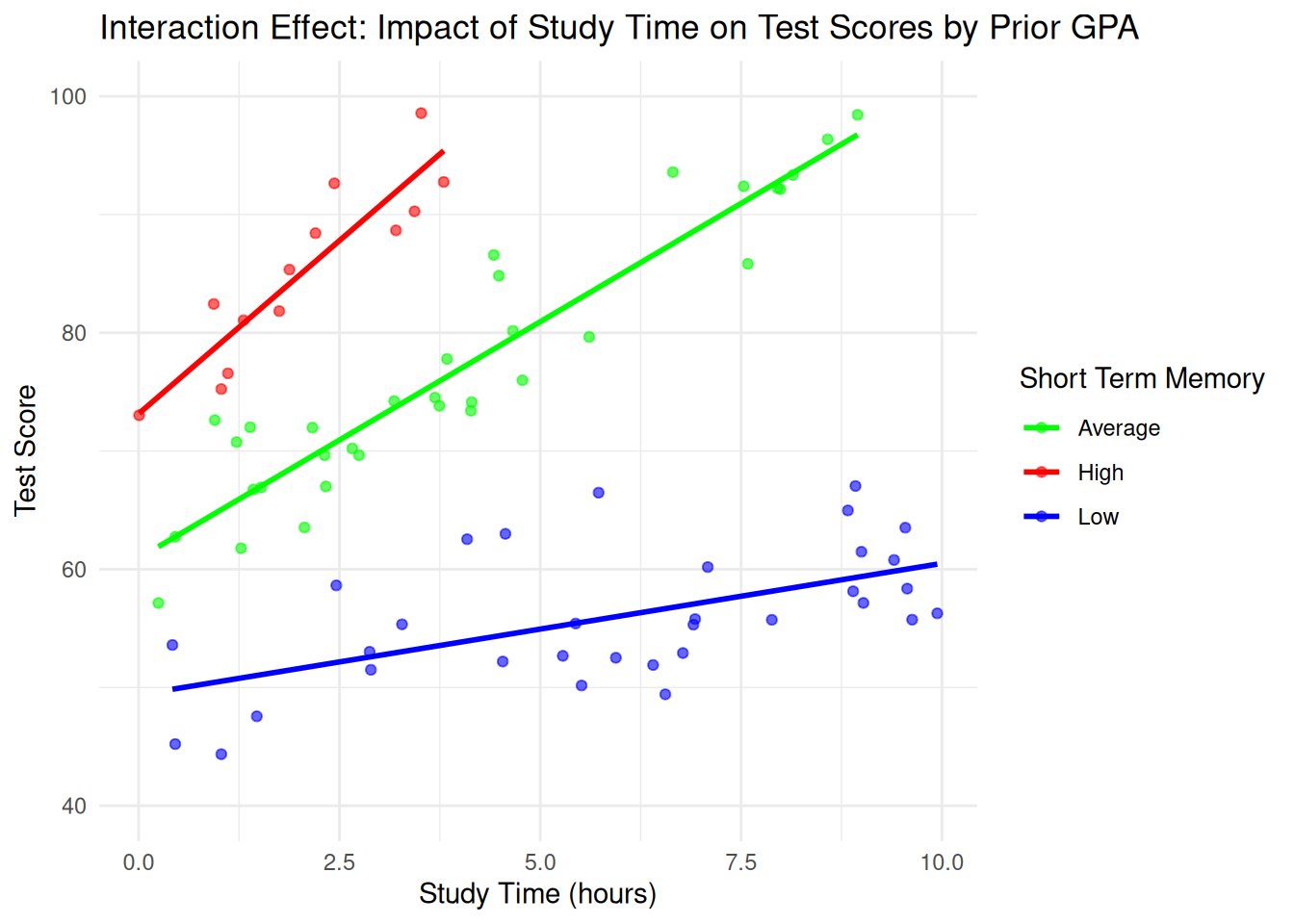
The following (fake) dataset represents what we might expect to see if we classified students according to their short term memory by some test (low, average, or high). We see that, in this dataset, students with “high” short term memories benefit from studying very rapidly, while students with low short term memories require more study time to increase their grade; the lines fit to the data points correspond to the least squares estimates of the relationship for each group.
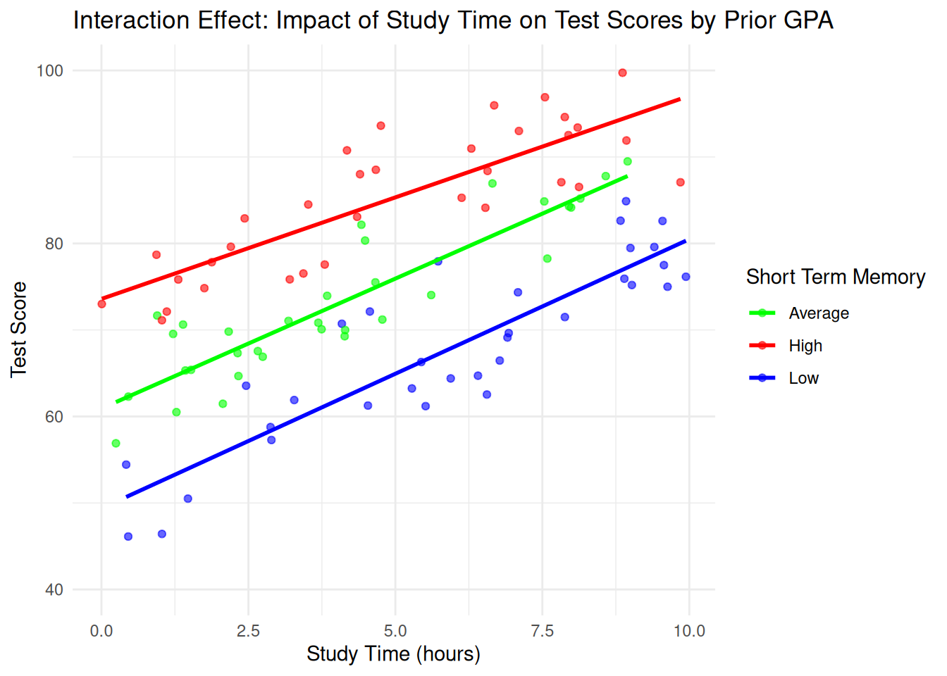
Contrast this with the following picture where students benefit from studying at the same rate regardless of their short term memory. In this figure, while those with high short term memories still tend to perform better, the benefit of studying an hour is 3 points per hour (on average) regardless of the group.
12.2 Real Example: GPA
It turns out on the GPA dataset that we have been looking at there is a potential interaction effect: high school GPA seems to be more informative as a predictor of first year GPA for men than women. This is demonstrated in the figure below:
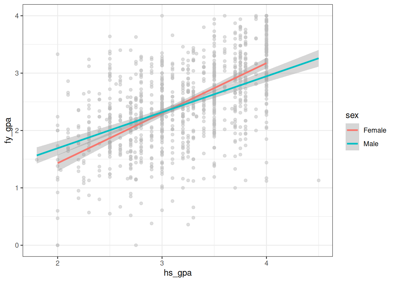
This figure plots two separate linear regressions with hs_gpa as the independent variable and fy_gpa as the dependent variable, but allowing for different lines for men and women. We see clearly in the figure that the slope for women is larger than the slope for men, suggesting that changes in hs_gpa for women tends to have a larger effect on fy_gpa than it does for men. In layman’s terms, the performance of women tends to be more consistent with their high school GPA than the performance of men.
To be a little bit more precise, we can see this from inspecting these two linear regressions:
fygpa_men <- lm(fy_gpa ~ hs_gpa, data = subset(fygpa, sex == "Male"))
fygpa_women <- lm(fy_gpa ~ hs_gpa, data = subset(fygpa, sex == "Female"))

summary(fygpa_men)
Call:
lm(formula = fy_gpa ~ hs_gpa, data = subset(fygpa, sex == "Male"))

Residuals:
     Min       1Q   Median       3Q      Max
-2.12900 -0.37048  0.03457  0.41771  1.68181

Coefficients:
            Estimate Std. Error t value Pr(>|t|)
(Intercept)  0.43656    0.15918   2.742  0.00631 **
hs_gpa       0.62721    0.05018  12.500  < 2e-16 ***
---
Signif. codes:  0 '***' 0.001 '**' 0.01 '*' 0.05 '.' 0.1 ' ' 1

Residual standard error: 0.6279 on 514 degrees of freedom
Multiple R-squared:  0.2331,    Adjusted R-squared:  0.2316
F-statistic: 156.2 on 1 and 514 DF,  p-value: < 2.2e-16
When just looking at men, we see from the \(R^2\) that hs_gpa accounts for about 23% of the variance in fy_gpa. For women, we instead get:
summary(fygpa_women)
Call:
lm(formula = fy_gpa ~ hs_gpa, data = subset(fygpa, sex == "Female"))

Residuals:
     Min       1Q   Median       3Q      Max
-2.08521 -0.34784  0.05184  0.42663  1.89865

Coefficients:
            Estimate Std. Error t value Pr(>|t|)
(Intercept) -0.31229    0.17695  -1.765   0.0782 .
hs_gpa       0.87182    0.05333  16.346   <2e-16 ***
---
Signif. codes:  0 '***' 0.001 '**' 0.01 '*' 0.05 '.' 0.1 ' ' 1

Residual standard error: 0.6097 on 482 degrees of freedom
Multiple R-squared:  0.3567,    Adjusted R-squared:  0.3553
F-statistic: 267.2 on 1 and 482 DF,  p-value: < 2.2e-16
So for women, we instead explain 36% of the variance in fy_gpa. This is a pretty big difference!
12.3 Modeling Interactions
Let’s begin by considering a model with two independent variables \(X_{i1}\) and \(X_{i2}\) in addition to \(Y_i\). A linear regression that includes an interaction between these variables is
\[ Y_i = \beta_0 + \beta_1 \, X_{i1} + \beta_2 X_{i2} + \beta_{3} \, (X_{i1} \times X_{i2}) + \epsilon_i. \]
What this amounts to, effectively, is including a third derived variable \(X_{i1} \times X_{i2}\) as a new predictor in the model. This term allows the effect of \(X_{i1}\) on \(Y_i\) to depend on \(X_{i2}\).
To interpret this model, we will rewrite the expression above slightly as:
\[ Y_i = (\beta_0 + \beta_2 \, X_{i2}) + (\beta_1 + \beta_3 \, X_{i2}) X_{i1} + \epsilon_i. \]
If we are thinking just about the effect of \(X_{i1}\) on \(Y_i\), then we might notice that (holding \(X_{i2}\) fixed) this is also a linear regression, with a new intercept \((\beta_0 + \beta_2 \, X_{i2})\) and slope \((\beta_1 + \beta_3 \, X_{i2})\). The key thing now is that the slope and intercept of this regression line depend on \(X_{i2}\)!
To connect this with our study time example, we might let \(X_{i1}\) represent study time and \(X_{i2}\) our short-term memory ability, and \(Y_i\) would be the test score. We could then interpret the \(\beta\)’s in the model as follows:
\(\beta_0\) is the intercept.
For a fixed value of \(X_{i2}\), a unit increase in \(X_{i1}\) increases the predicted value of \(Y_i\) by \(\beta_1 + \beta_3 \, X_{i2}\). The slope \(\beta_1\) now represents the effect of \(X_{i1}\) on \(Y_i\) when \(X_{i2}\) takes the particular value of \(0\).
For a fixed value of \(X_{i1}\), a unit increase in \(X_{i2}\) increases the predicted value of \(Y_i\) by \(\beta_2 + \beta_3 \, X_{i1}\). As above, \(\beta_2\) is now the effect of \(X_{i2}\) on \(Y_i\) when \(X_{i1}\) takes the particular value \(0\).
12.4 Interaction Terms With Categorical Variables
There is no restriction on which types of independent variables you can use in your interactions: they can be numeric or categorical. A nice thing about using categorical variables in interactions is that the interpretations can be pretty simple: for each level of my categorical variable, I basically get a different regression line!
For a categorical variable with two levels (like sex in the GPA dataset), the interaction model can be written as
\[ \texttt{fy\_gpa}_i = \beta_0 + \beta_1 \, \texttt{hs\_gpa}_i + \beta_2 \, \texttt{sex}_i + \beta_3 \, (\texttt{hs\_gpa}_i \times \texttt{sex}_i) + \epsilon_i \]
where recall that sex is 1 if the student is male and 0 otherwise. This model effectively fits two separate lines: one for males and one for females. For females, (sex = 0) we have the line
\[ \texttt{fy\_gpa}_i = \beta_0 + \beta_1 \, \texttt{hs\_gpa}_i + \epsilon_i \]
while for males we have the line
\[ \texttt{fy\_gpa}_i = (\beta_0 + \beta_2) + (\beta_1 + \beta_3) \, \texttt{hs\_gpa}_i + \epsilon_i. \]
In this formulation:
- \(\beta_0\) is the intercept for females .
- \(\beta_1\) is the slope for females - \(\beta_0 + \beta_2\) is the intercept for males .
- \(\beta_1 + \beta_3\) is the slope for males.
- Therefore, \(\beta_2\) is the difference in intercepts for males and females, while \(\beta_3\) is the difference in slopes for males.
12.4.1 More Than Two Levels
For categorical variables with more than two levels, the process is similar but involves multiple dummy variables. To illustrate, we’ll use the Palmer Penguins dataset, which contains measurements on three species of Penguins (Adelie, Gentoo, and Chinstrap penguins) living on three islands:
library(palmerpenguins)
head(penguins)
# A tibble: 6 × 8
species island bill_length_mm bill_depth_mm flipper_length_mm body_mass_g
<fct> <fct> <dbl> <dbl> <int> <int>
1 Adelie Torgersen 39.1 18.7 181 3750
2 Adelie Torgersen 39.5 17.4 186 3800
3 Adelie Torgersen 40.3 18 195 3250
4 Adelie Torgersen NA NA NA NA
5 Adelie Torgersen 36.7 19.3 193 3450
6 Adelie Torgersen 39.3 20.6 190 3650
# ℹ 2 more variables: sex <fct>, year <int>unique(penguins$species)[1] Adelie Gentoo Chinstrap
Levels: Adelie Chinstrap GentooWe’ll look at predicting the body mass of a penguin from their bill length. Below, we plot the data along with a separate linear regression for each of the species:
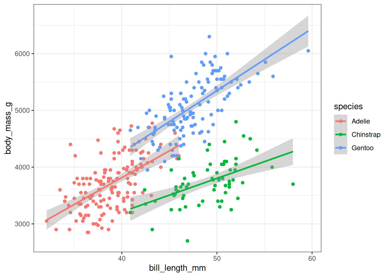
We might expect that, for whatever reason, the relationship between bill length and body mass might itself depend on the species of the penguin. Accordingly, we can fit the following model:
\[ \begin{aligned} \texttt{body\_mass}_i = &\beta_0 + \beta_1 \, \texttt{bill\_length}_i \\ &+ \beta_2 \, \texttt{species\_Chinstrap}_i + \beta_3 \, \texttt{species\_Gentoo}_i \\ &+ \beta_4 \, (\texttt{bill\_length}_i \times \texttt{species\_Chinstrap}_i) \\ &+ \beta_5 \, (\texttt{bill\_length}_i \times \texttt{species\_Gentoo}_i) + \epsilon_i \end{aligned} \]
where \(\texttt{species\_Chinstrap}_i\) is 1 if the \(i\)-th penguin is a Chinstrap and 0 otherwise, and \(\texttt{species\_Gentoo}_i\) is defined similarly. This model effectively fits three separate lines: one for each species of penguin. For Adelie penguins (the reference category), we have the line:
\[ \texttt{body\_mass}_i = \beta_0 + \beta_1 \, \texttt{bill\_length}_i + \epsilon_i \]
For Chinstrap penguins, we have:
\[ \texttt{body\_mass}_i = (\beta_0 + \beta_2) + (\beta_1 + \beta_4) \, \texttt{bill\_length}_i + \epsilon_i \]
And for Gentoo penguins:
\[ \texttt{body\_mass}_i = (\beta_0 + \beta_3) + (\beta_1 + \beta_5) \, \texttt{bill\_length}_i + \epsilon_i \]
Interpreting these coefficients, we have:
- \(\beta_0\) is the intercept for Adelie penguins (the reference category).
- \(\beta_1\) is the slope relating bill length to body mass for Adelie penguins.
- \(\beta_2\) represents how much higher (or lower) the intercept is for Chinstrap penguins compared to Adelie penguins.
- \(\beta_3\) represents how much higher (or lower) the intercept is for Gentoo penguins compared to Adelie penguins.
- \(\beta_4\) represents how much the slope for Chinstrap penguins differs from the slope for Adelie penguins. In other words, it’s the additional effect of bill length on body mass specific to Chinstrap penguins.
- \(\beta_5\) represents how much the slope for Gentoo penguins differs from the slope for Adelie penguins. In other words, it’s the difference in the effect of bill length on body mass for Gentoo penguins compared to Adelie penguins.
This model allows us to capture not only the differences in average body mass between species (through \(\beta_2\) and \(\beta_3\)) but also how the relationship between bill length and body mass varies across species (through \(\beta_4\) and \(\beta_5\)).
12.4.2 How Does This Differ from Just Doing Separate Regressions?
At the beginning of this chapter we motivated the concept of interactions by fitting two separate regressions: one for men and one for women. It seems like this is basically the same thing as what we have been doing when considering interactions with categorical variable, as we also get two separate regression lines.
To some extent, there isn’t much of a difference, at least when we have one numeric variable and one categorical variable. The estimated lines turn out to be equivalent. Below, we discuss some ways in which the two approaches still differ.
Different residual standard errors: The most salient difference between the two approaches is that, when a single regression with an interaction is used, we implicitly assume that \(\sigma\) (i.e., the standard deviation of the error) is the same for both males and females, whereas if we use two separate regressions then we implicitly assume that \(\sigma\) is different.
It turns out, at least in the case of the GPA dataset, that the residual standard error is very similar across men and women:
sigma(fygpa_men)[1] 0.6278814sigma(fygpa_women)[1] 0.6096951More Variables: The equivalence no longer holds once we start going beyond a single numeric and categorical predictor. For example, if we consider the model
\[ \texttt{fy\_gpa}_i = \beta_0 + \beta_1 \, \texttt{hs\_gpa}_i + \beta_2 \, \texttt{sex}_i + \beta_3 \, (\texttt{hs\_gpa}_i \times \texttt{sex}_i) + \beta_4 \, \texttt{sat\_m}_i + \epsilon_i \]
then we can no longer obtain this model by fitting separate regressions for males and females. The reason this doesn’t work is that the above model does not include an interaction between SAT math score and sex, whereas fitting separate regressions for males and females would effectively include such an interaction.
12.5 Always Include Main Effects of an Interaction
When constructing models with interactions, the standard practice is to not include an interaction in your model if you are not including the associated main effects. For example, for the GPA data, we would not consider the following model:
\[ \texttt{fy\_gpa}_i = \beta_0 + \beta_1 \, \texttt{sex}_i + \beta_2 (\texttt{hs\_gpa}_i \times \texttt{sex}_i) + \epsilon_i \]
The reason we would not consider this model is because it includes an interaction term (high school GPA and sex) without including an associated main effect (the main effect of high school GPA is missing). We can fix this issue by using a model that includes the main effect of high school GPA as well.
Why do we do this? Here are a couple of reasons:
- In real world datasets, it is exceedingly rare for there to exist an interaction without a main effect. It’s not impossible, but it is rare enough that the default is to include the main effects.
- The model without the main effect imposes some odd restrictions on the model. For example, in this case it implies that high school GPA is relevant for men, but not for women. We can avoid this (and other) weirdness in the interpretation of interactions by just defaulting to always including the main effects.
In practice, there are rare occasions where theory might suggest omitting a main effect. However, such decisions should be made with extreme caution and strong theoretical justification.
12.6 Higher Order Interactions
So far, we’ve focused on interactions between two variables. However, in some cases, the relationship between variables can be even more complex, involving three or more variables. These are called higher-order interactions.
A three-way interaction occurs when the relationship between two variables depends on the level of a third variable. Mathematically, for variables \(X_1\), \(X_2\), and \(X_3\), a model with a three-way interaction can be written as:
\[ Y_i = \beta_0 + \beta_1X_{1i} + \beta_2X_{2i} + \beta_3X_{3i} + \beta_4(X_{1i}X_{2i}) + \beta_5(X_{1i}X_{3i}) + \beta_6(X_{2i}X_{3i}) + \beta_7(X_{1i}X_{2i}X_{3i}) + \epsilon_i \]
Note that this model includes all lower-order terms (main effects and two-way interactions) in addition to the three-way interaction term \(X_{1i}X_{2i}X_{3i}\).
12.6.1 Interpreting Three-Way Interactions
Interpreting three-way interactions can be challenging. One way to think about it is that the two-way interaction between any two variables changes depending on the level of the third variable.
For example, let’s consider a hypothetical study on the effect of a new drug on blood pressure, where we’re interested in how the drug’s effect might vary based on both the patient’s age and sex. Our variables could be:
- \(X_1\): Drug dosage (numeric)
- \(X_2\): Age (numeric)
- \(X_3\): Sex (categorical: 0 for female, 1 for male)
- \(Y\): Change in blood pressure
A significant three-way interaction might indicate that the interaction between drug dosage and age on blood pressure change is different for males and females.
12.6.2 Reason to Avoid Higher Order Interactions
As a general rule, there is a preference for simpler models with straightforward interpretations. To the extent that three-way (and higher) interactions are difficult to interpret, this is a reason to avoid them. Ideally, when considering higher-order interactions we prefer for there to be some plausible scientific explanation for why we should expect them to occur.
Another reason to avoid higher order interactions is that they are usually quite small, so that the model is not much better if you include them. Because they are often so small, it can take large amounts of data to estimate them with any sort of reasonable precision. A side effect of this is that models with higher-order interactions can often make very strange predictions when you extrapolate even just a little bit beyond the range of the data.
Finally, if you start including interactions capriciously, there is a risk of overfitting the data. We will talk about overfitting in more detail in a later chapter, but essentially the cause of overfitting is including too many variables (i.e., making your \(P\) large) when you do not have enough observations (i.e., your \(N\) is not big enough).
In my experience, second order interactions are relatively common, third order interactions are quite uncommon, and I personally have never seen a serious use of a fourth order interaction in a vanilla linear regression in my life. That’s not to say that fourth-and-higher order interactions never appear, but they are generally associated with more advanced techniques that we will not learn about in this course (such as classification and regression trees, neural networks, and kernel methods).
12.7 Fitting a Model With Interactions in R
In R, we can fit models with interaction terms using the lm() function; we just need to specify that there is an interaction in the model formula. Using the GPA dataset to demonstrate the process, we can include an interaction between hs_gpa and sex as follows:
fygpa_interaction <- lm(fy_gpa ~ hs_gpa * sex, data = fygpa)Rather than using a + symbol to specify the model, we instead use a * symbol. This fits the model
\[ \texttt{fy\_gpa}_i = \beta_0 + \beta_1 \, \texttt{hs\_gpa}_i + \beta_2 \, \texttt{sex}_i + \beta_3 \, (\texttt{hs\_gpa}_i \times \texttt{sex}_i) + \epsilon_i \]
Note that this automatically includes the main effects. Printing the summary we have
summary(fygpa_interaction)
Call:
lm(formula = fy_gpa ~ hs_gpa * sex, data = fygpa)

Residuals:
     Min       1Q   Median       3Q      Max
-2.12900 -0.36526  0.04206  0.42470  1.89865

Coefficients:
               Estimate Std. Error t value Pr(>|t|)
(Intercept)    -0.31229    0.17970  -1.738 0.082546 .
hs_gpa          0.87182    0.05416  16.097  < 2e-16 ***
sexMale         0.74884    0.23860   3.138 0.001748 **
hs_gpa:sexMale -0.24461    0.07336  -3.334 0.000887 ***
---
Signif. codes:  0 '***' 0.001 '**' 0.01 '*' 0.05 '.' 0.1 ' ' 1

Residual standard error: 0.6191 on 996 degrees of freedom
Multiple R-squared:  0.3036,    Adjusted R-squared:  0.3015
F-statistic: 144.7 on 3 and 996 DF,  p-value: < 2.2e-16
Looking at this output, we see that the interaction between sex and high school GPA is highly statistically significant, i.e., there appears to be an interaction between these variables in predicting college GPA. In more detail:
- The coefficient for
hs_gpa(0.87182) represents the effect of high school GPA on first-year GPA for females (the reference category forsex). - The coefficient for
sexMale(0.74884) represents the difference in the predicted college GPAs between males and females whenhs_gpais zero (which is an extrapolation and probably not meaningful in this context). - The interaction term
hs_gpa:sexMale(-0.24461) indicates how the effect of high school GPA differs for males compared to females. The negative value suggests that the effect of high school GPA on first-year GPA is smaller for males than for females.
For simple models with just an interaction between a single categorical variable (sex) and numeric variable (high school GPA), we can also quickly visualize things using the qplot() function in the ggplot2 package:
library(ggplot2)
qplot(x = hs_gpa, y = fy_gpa, color = sex, data = fygpa) + geom_smooth(method = 'lm')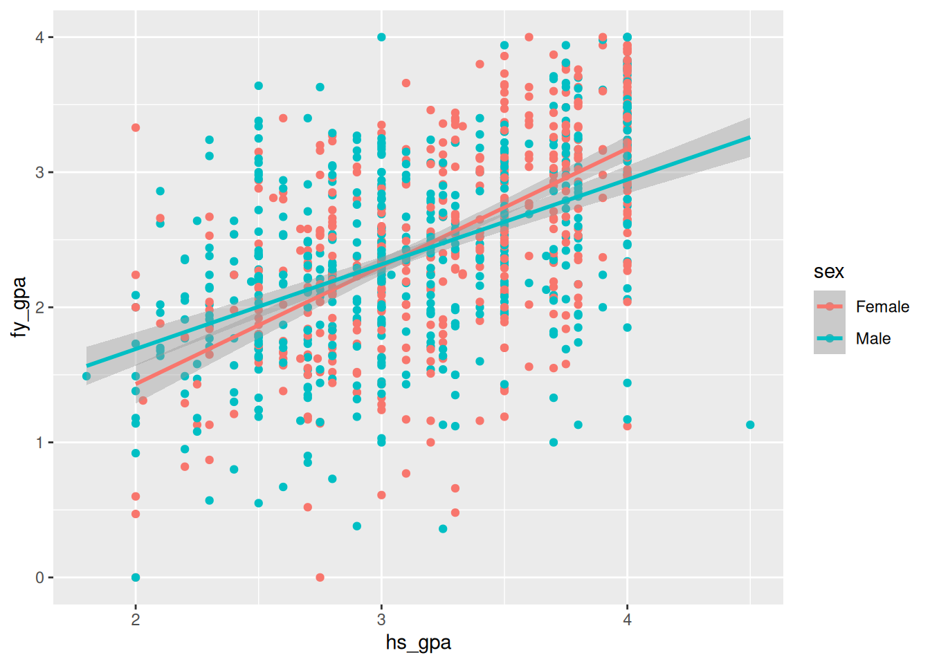
We can also compare this model with the main effects model (without interaction) using the anova() function for comparing nested models:
fygpa_sex_hs <- lm(fy_gpa ~ hs_gpa + sex, data = fygpa)
anova(fygpa_sex_hs, fygpa_interaction)
Analysis of Variance Table
Model 1: fy_gpa ~ hs_gpa + sex
Model 2: fy_gpa ~ hs_gpa * sex
Res.Df RSS Df Sum of Sq F Pr(>F)
1 997 386.07
2 996 381.81 1 4.2619 11.118 0.0008866 ***
---
Signif. codes: 0 '***' 0.001 '**' 0.01 '*' 0.05 '.' 0.1 ' ' 1In view of the low \(P\)-value, we can conclude that there is evidence supporting that the interaction term improves the fit of the regression to the data.
We can also add other variables into the mix. For example, let’s say we want to include SAT math score, and we want this variable to interact with sex, but we do not want SAT math score to interact with high school GPA. We can do this with the following model:
fygpa_interaction_2 <- lm(fy_gpa ~ hs_gpa * sex + sat_m * sex, data = fygpa)
summary(fygpa_interaction_2)
Call:
lm(formula = fy_gpa ~ hs_gpa * sex + sat_m * sex, data = fygpa)

Residuals:
     Min       1Q   Median       3Q      Max
-2.19531 -0.36159  0.03465  0.40996  1.75451

Coefficients:
                Estimate Std. Error t value Pr(>|t|)
(Intercept)    -0.802745   0.205518  -3.906 0.000100 ***
hs_gpa          0.756401   0.058370  12.959  < 2e-16 ***
sexMale         0.283956   0.286523   0.991 0.321906
sat_m           0.016643   0.003736   4.455 9.35e-06 ***
hs_gpa:sexMale -0.292513   0.078637  -3.720 0.000211 ***
sexMale:sat_m   0.009315   0.005140   1.812 0.070230 .
---
Signif. codes:  0 '***' 0.001 '**' 0.01 '*' 0.05 '.' 0.1 ' ' 1

Residual standard error: 0.5979 on 994 degrees of freedom
Multiple R-squared:  0.3518,    Adjusted R-squared:  0.3485
F-statistic: 107.9 on 5 and 994 DF,  p-value: < 2.2e-16
We see that the above model includes (i) all of the main effects, (ii) an interaction between sex and high school GPA, and (iii) an interaction between sex and SAT math.
12.7.1 Three-Way Interactions
Let’s now consider a model with a three-way interaction between high school GPA, sex, and SAT math score. This model would be written
\[ \begin{aligned} \texttt{fy\_gpa}_i = &\beta_0 + \beta_1 \, \texttt{hs\_gpa}_i + \beta_2 \, \texttt{sex}_i + \beta_3 \, \texttt{sat\_m}_i \\ &+ \beta_4 \, (\texttt{hs\_gpa}_i \times \texttt{sex}_i) \\ &+ \beta_5 \, (\texttt{hs\_gpa}_i \times \texttt{sat\_m}_i) \\ &+ \beta_6 \, (\texttt{sex}_i \times \texttt{sat\_m}_i) \\ &+ \beta_7 \, (\texttt{hs\_gpa}_i \times \texttt{sex}_i \times \texttt{sat\_m}_i) + \epsilon_i \end{aligned} \]
This model includes all main effects, all two-way interactions, and the three-way interaction between high school GPA, sex, and SAT math score.
We can fit this model in R by running
fygpa_threeway <- lm(fy_gpa ~ hs_gpa * sat_m * sex , data = fygpa)And we can quickly assess whether the three-way interaction is needed from the summary:
summary(fygpa_threeway)
Call:
lm(formula = fy_gpa ~ hs_gpa * sat_m * sex, data = fygpa)

Residuals:
     Min       1Q   Median       3Q      Max
-2.17571 -0.36407  0.02109  0.40444  1.77864

Coefficients:
                      Estimate Std. Error t value Pr(>|t|)
(Intercept)           1.320737   1.057972   1.248   0.2122
hs_gpa                0.096168   0.327930   0.293   0.7694
sat_m                -0.024666   0.020532  -1.201   0.2299
sexMale               1.553455   1.441406   1.078   0.2814
hs_gpa:sat_m          0.012701   0.006209   2.046   0.0411 *
hs_gpa:sexMale       -0.738965   0.456126  -1.620   0.1055
sat_m:sexMale        -0.009862   0.026943  -0.366   0.7144
hs_gpa:sat_m:sexMale  0.006814   0.008304   0.821   0.4121
---
Signif. codes:  0 '***' 0.001 '**' 0.01 '*' 0.05 '.' 0.1 ' ' 1

Residual standard error: 0.5936 on 992 degrees of freedom
Multiple R-squared:  0.3625,    Adjusted R-squared:  0.358
F-statistic: 80.59 on 7 and 992 DF,  p-value: < 2.2e-16
We see that there is not much evidence favoring the three-way interaction after including all of the main effects and two-way interactions (\(P\)-value of 0.4121). We can also look at the sequential \(F\)-tests to see where we stop needing to increase the model’s complexity:
anova(fygpa_threeway)Analysis of Variance Table
Response: fy_gpa
Df Sum Sq Mean Sq F value Pr(>F)
hs_gpa 1 161.86 161.860 459.4206 < 2.2e-16 ***
sat_m 1 21.12 21.117 59.9383 2.407e-14 ***
sex 1 4.92 4.921 13.9682 0.0001965 ***
hs_gpa:sat_m 1 3.12 3.115 8.8423 0.0030145 **
hs_gpa:sex 1 5.63 5.631 15.9820 6.869e-05 ***
sat_m:sex 1 1.87 1.869 5.3042 0.0214796 *
hs_gpa:sat_m:sex 1 0.24 0.237 0.6733 0.4120939
Residuals 992 349.49 0.352
---
Signif. codes: 0 '***' 0.001 '**' 0.01 '*' 0.05 '.' 0.1 ' ' 1We see that there is actually quite a bit of support for each of the other main effects and interactions when building up the model sequentially, with the exception of the three-way interaction.
12.8 Exercises
12.8.1 Boston Again
We again revisit the Boston housing dataset, where our interest is in understanding the relationship between the concentration of nitric oxide in a census tract (nox) and the median home value in that tract. First, we load the data:
Boston <- MASS::Boston
head(Boston)
crim zn indus chas nox rm age dis rad tax ptratio black lstat
1 0.00632 18 2.31 0 0.538 6.575 65.2 4.0900 1 296 15.3 396.90 4.98
2 0.02731 0 7.07 0 0.469 6.421 78.9 4.9671 2 242 17.8 396.90 9.14
3 0.02729 0 7.07 0 0.469 7.185 61.1 4.9671 2 242 17.8 392.83 4.03
4 0.03237 0 2.18 0 0.458 6.998 45.8 6.0622 3 222 18.7 394.63 2.94
5 0.06905 0 2.18 0 0.458 7.147 54.2 6.0622 3 222 18.7 396.90 5.33
6 0.02985 0 2.18 0 0.458 6.430 58.7 6.0622 3 222 18.7 394.12 5.21
medv
1 24.0
2 21.6
3 34.7
4 33.4
5 36.2
6 28.7Familiarize yourself with the data by running ?MASS::Boston in the console. In addition to nox and medv, we will consider a number of additional factors that are relevant for predicting medv.
Fit a model to the dataset using the formula
medv ~ nox * dis + lstat. Describe in words the model being fitted (i.e., which interactions and main effects are included).Repeat part (a), but use the formula
medv ~ nox * dis + nox * lstat.Based on the output of
summaryfor these models, does the evidence suggest that the additional interaction term(s) of the part (b) model are necessary when compared to the model from part (a)? Explain.Based on the output of
summaryon part (b), does the evidence suggest that all of the main effects (nox,dis, andlstat) are needed for predictingmedv?Interpret the interaction between
noxanddisin part (a), in terms of how changingnoxcauses the effect ofdisonmedvto change.Interpret the interaction between
noxanddisin part (a), in terms of how changingdiscauses the effect ofnoxonmedvto change.
12.8.2 Palmer Penguins
For this exercise, you will get to play with the Palmer Penguins dataset. This dataset can be loaded by running the following commands:
## Run install.packages("palmerpenguins") to install the package
library(palmerpenguins)
head(penguins)
# A tibble: 6 × 8
species island bill_length_mm bill_depth_mm flipper_length_mm body_mass_g
<fct> <fct> <dbl> <dbl> <int> <int>
1 Adelie Torgersen 39.1 18.7 181 3750
2 Adelie Torgersen 39.5 17.4 186 3800
3 Adelie Torgersen 40.3 18 195 3250
4 Adelie Torgersen NA NA NA NA
5 Adelie Torgersen 36.7 19.3 193 3450
6 Adelie Torgersen 39.3 20.6 190 3650
# ℹ 2 more variables: sex <fct>, year <int>Run ?penguins in the console to learn more about this dataset. Our interest will be in a potential three-way interaction between sex, species, and flipper_length_mm in predicting body_mass_g.
Fit a model that includes a three-way interaction between sex, species, and flipper length for predicting body mass. Using the output of
summary, perform an overall \(F\)-test for significance of the model (report the \(P\)-value and what you can conclude from it).Apply the
anovafunction to the model you fit from part (a). Use the results to assess whether or not there is evidence for the two-way and three-way interaction effects.Use the
predictfunction to get predictions for thefemaleandmalepenguins for each of the three species (Adelie,Chinstrap,Gentoo) for the values offlipper_length_mmalong the following grid:flipper_length_grid <- seq(from = 172, to = 231, length = 50)Then plot the predictions against
flipper_length_grid, coloring the points differently for each combination of sex and species.Using the output of
summary, write down an estimated model of the form\[ \texttt{body\_mass\_g} = \beta_0 + \beta_1 \, \texttt{flipper\_length\_mm} + \text{error}_i \]
specifically for the group of male Chinstrap penguins. (That is, fill in the missing values of \(\beta_0\) and \(\beta_1\) below with numerical values.)
Now, using
lm, fit a linear model specifically to the data subset containing only male Chinstrap penguins. That is, create a new dataset consisting of just this subgroup, and fit a linear regression ofbody_mass_gonflipper_length_mm. How do the results here compare with the results on part (d)?Are there any ways in which the model fit in part (e) differs from the fit of the full model? That is, do we get exactly the same results in all respects?
12.8.3 Wages
13 Exercise: Wages
The following problem revisits the Wage dataset from the ISLR package, where our interest is in understanding the relationship between wage and age, controlling for amount of education. First, we load the data:
## Install the ISLR package if you do not have it
wage <- ISLR::Wage
head(wage)
year age maritl race education region
231655 2006 18 1. Never Married 1. White 1. < HS Grad 2. Middle Atlantic
86582 2004 24 1. Never Married 1. White 4. College Grad 2. Middle Atlantic
161300 2003 45 2. Married 1. White 3. Some College 2. Middle Atlantic
155159 2003 43 2. Married 3. Asian 4. College Grad 2. Middle Atlantic
11443 2005 50 4. Divorced 1. White 2. HS Grad 2. Middle Atlantic
376662 2008 54 2. Married 1. White 4. College Grad 2. Middle Atlantic
jobclass health health_ins logwage wage
231655 1. Industrial 1. <=Good 2. No 4.318063 75.04315
86582 2. Information 2. >=Very Good 2. No 4.255273 70.47602
161300 1. Industrial 1. <=Good 1. Yes 4.875061 130.98218
155159 2. Information 2. >=Very Good 1. Yes 5.041393 154.68529
11443 2. Information 1. <=Good 1. Yes 4.318063 75.04315
376662 2. Information 2. >=Very Good 1. Yes 4.845098 127.11574If necessary, familiarize yourself with the data by running ?ISLR::Wage in the console.
Fit linear models defined by the following formulas:
wage ~ age * educationlogwage ~ age + educationlogwage ~ age * education
Using the
autoplotfunction applied to these fits, which of the models seems to do the best job at satisfying the standard assumptions of the linear regression model? Explain your answer.What model does
lm(logwage ~ poly(age, 4) * education, data = wage)fit? Explain, in words, what model is being fit for each level of education, and how this model would differ from the model that setslm(logwage ~ poly(age, 4) + education, data = wage).For the model
lm(logwage ~ poly(age, 4) * education, data = wage), plot age on the x axis against the outcome on the y axis. Using thelinesandpredictfunctions, plot a separate curve associated to the predicted wage for each level of education. Explain, qualitatively, how education affects the relationship between age and wage, focusing on how the wages differ for young people versus how they differ for middle aged people.Using adjusted \(R^2\), identify the optimal value of
kinpoly(age,k)for predictinglogwagefromageandeducation. How does this compare to the optimal number knots in a spline fit withns(age, df = k)? (Revisit the lecture video and notes for a refresher on splines.)