4 * 3 + 2 ## Equals 14, not 20[1] 144 * (3 + 2) ## Now, we do addition first[1] 20In this course, we will do our statistical analyses using the RStudio software. The first order of business for you is to do the following:
Download and install R from https://cloud.r-project.org/. Follow the instructions there.
Download and install RStudio from https://posit.co/download/rstudio-desktop/. Again, follow the instructions there.
A video lesson showing how to do this is available here.
For this course, there is an online RStudio server you can also use, and I will show you in class how to use it.
I recommend that you organize your homework/notes/etc for this course in a RStudio Project. This will help you keep track of all of your files and ensure that your R session is always working in the appropriate directory of your computer. I do not require that you do this, it just seems like a good idea.
If you have occasion to use RStudio outside of this course, I recommend that you use separate project files for all of your projects.
Benefits of using projects include:
You can create a new project by clicking File->New Project. Then, select New Directory, New Project, and give your project a name and location. This will create a new folder in the location with the given name.
After making the project, it will open automatically in your session. You will also be able to open the project in future sessions in a few different ways:
your_project_name.RProj to open an RStudio session with the project.Files you create and save will now automatically be added to this folder, and all file paths will be relative to the project location. I recommend you save datasets for this class in this folder as well.
SDS324E on your computer.satgpa.csv dataset from this link and save it to your project directory.We can interact with R directly by typing commands into the RStudio console pane and pressing the Enter (or Return) key to run the commands. A picture of the console with some commands typed in is given below:
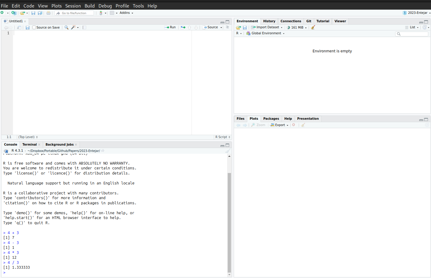
Notice that we can use the R console like a calculator for adding, subtracting, multiplying, and dividing numbers. The output of these commands appears on the lines with a [1] appearing (more on what the [1] means later). R respects the usual order of operations, so for example we have
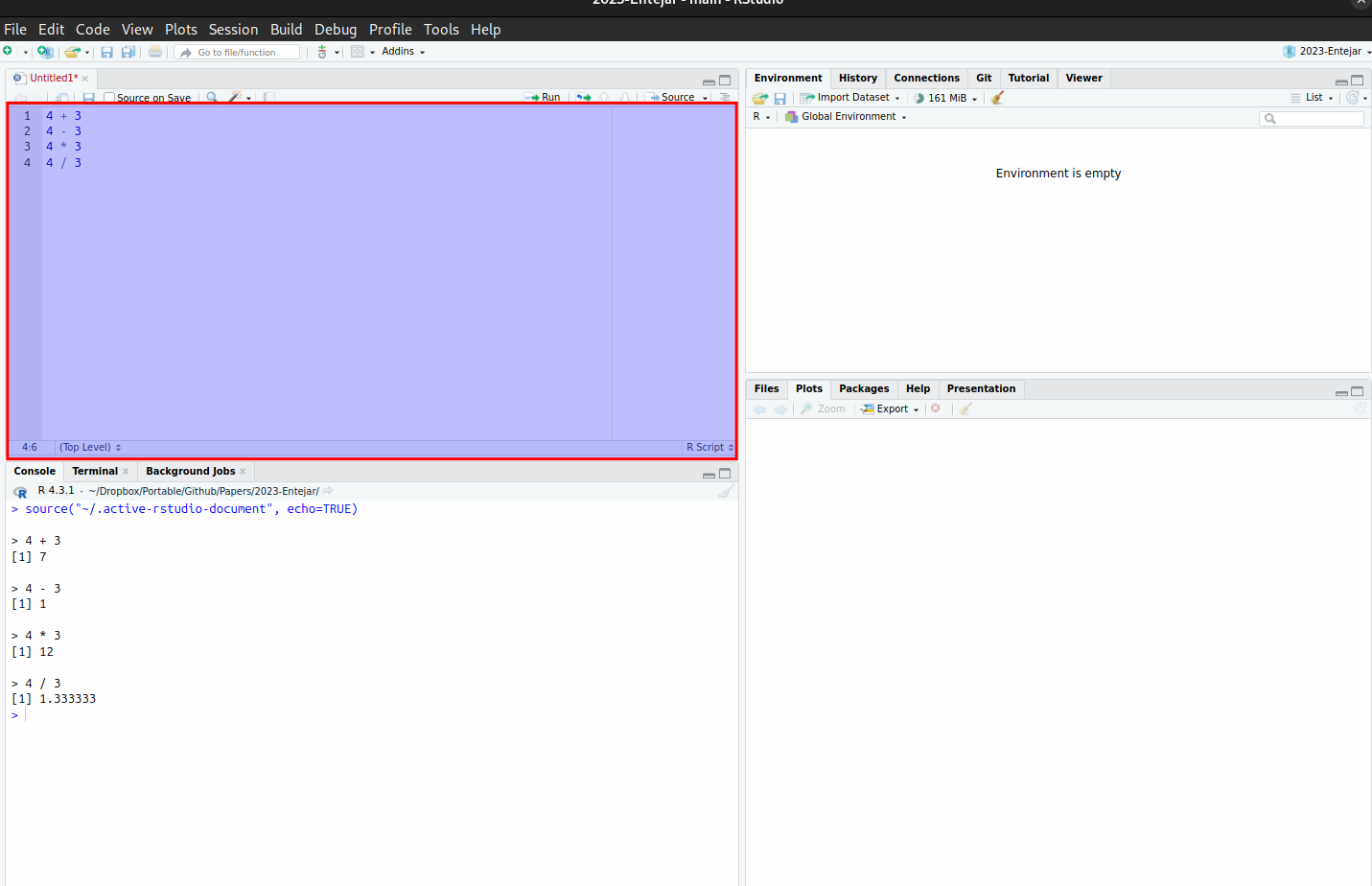
4 * 3 + 2 ## Equals 14, not 20[1] 144 * (3 + 2) ## Now, we do addition first[1] 20The console is useful for quick calculations, but we generally prefer to write our R commands in a script so that it can be reused. An R script can be used to write many commands that can be saved and executed in RStudio. This is particularly useful for reproducing results and handling complex analyses that require running multiple commands. To write a script, open RStudio and go to File -> New File -> R Script. This opens a new script tab where you can type R commands. Scripts can be written in the RStudio editor and saved with the .R extension, and can be executed all at once by clicking on the source button:
We can also run the code line-by-line using Ctrl + Enter (Windows) or Command + Return (Mac). The ability to reuse R analyses as scripts is essential for projects that involve complicated workflows or that need to be shared with others. After writing your script, save it by going to File -> Save.
We can add non-code text to an R script to help explain in the the script what the individual commands to. These text descriptions are referred to as comments, and can make a script much easier to read and understand for both others and future-you. A comment can be added using the # symbol; all text after the # symbol will be ignored when the code is executed. For example:
# This is a comment explaining the following line: computing 2 + 2
2 + 2
[1] 4Assignments for these notes are distributed as Quarto files, which have the qmd extension .qmd. Quarto is an open-source scientific and technical publishing system that allows you to create dynamic documents by combining text, code, and visualizations. For a detailed tutorial on Quarto, see this page. To use Quarto documents in RStudio:
Open RStudio and create a document by going to File -> New File -> Quarto Document.
Choose an output type which in this course will be an html file.
I recommend using the visual editor for editing Quarto documents, in which case sections, bullet points, etc. can be made using the bar at the top:
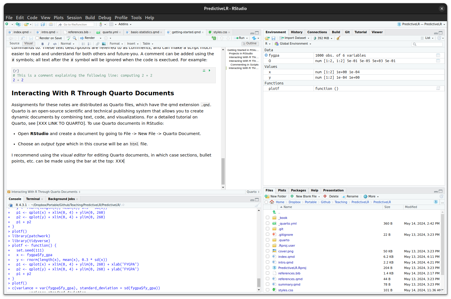
Quarto allows you to mix writing with code seamlessly. Code chunks can be inserted by starting a line with ```{r} or by clicking Insert -> Executable Cell -> R. To render a Quarto document and see the output, click the Render button. This executes all the code chunks and compiles the document into (say) an HTML file. The code is executed every time the document is rendered, so the output always reflects the current state of the code. Render early and often when working on assignments.
A common trap students fall into is running analyses in the console or a script that isn’t reflected in their Quarto document, so when they compile the document there are pieces of code missing from the execution; for example, maybe a dataset is loaded manually by the student, but the code for loading the dataset is not in the Quarto document, so when the document is compiled the data cannot be found. Quarto documents are compiled in an independent R session that does not have access to any of the variables in your environment!!!
The simplest thing R can do is function more-or-less like a calculator. For example, we can add/multiple/subtract/divide the numbers 2 and 3 by running
2 + 3[1] 52 * 3[1] 62 - 3[1] -12 / 3[1] 0.6666667Like using the memory inside a calculator, we can also store results inside of variables, as in
x <- 2 + 3
y <- 2 * 3

print(x)
[1] 5print(y)[1] 6Vectors provide a simple way to manipulate variables of the same type (i.e., numeric, character, factor, or logical variables). Vectors also are the building blocks of more advanced data structures in R (such as data frames, which hold entire datasets).
To create a vector in R, we use the c() function:
z <- c(1, 2, 3, 4, 5)
print(z)
[1] 1 2 3 4 5We see that z effectively contains the list of numbers from 1 to 5. We can also create vectors of other types. Strings, for example, are sequences of characters used to represent textual data, and are enclosed in quotation marks:
w <- c("red", "blue", "green")
print(w)
[1] "red" "blue" "green"We can also store true/false values (called boolean or logical vectors):
b <- c(TRUE, FALSE, FALSE, TRUE)
print(b)
[1] TRUE FALSE FALSE TRUEThe keywords TRUE and FALSE are reserved by the system to represent logical values. The c() function can also be used to glue vectors together as in
z2 <- c(6, 7, 8)
c(z, z2)
[1] 1 2 3 4 5 6 7 8After creating a vector, we can access the elements of the vector (i.e., the values stored inside the vector) using the square brackets []. For, for example, w[2] pulls out the second value of w:
w[2][1] "blue"It is also possible to pull out multiple elements at the same time by using a vector index. For example, we can use a logical vector to access elements of the vector as in
q <- c(3, 4, 5, 6)
q[c(FALSE, TRUE, FALSE, TRUE)]
[1] 4 6or we can use a numeric vector to access elements of the vector as in
q[c(2,3)][1] 4 5Often we want to grab just the first few elements of a vector. For example, maybe we just want the first three elements of q. We could do this by running q[c(1, 2, 3)], but fortunately there is a shortcut:
q[1:3][1] 3 4 5This works because 1:3 is shorthand for the vector c(1,2,3):
print(1:3)[1] 1 2 3While you don’t really need this for accessing just the first three, this is very convenient if you need (say) the first 100, since we can just type 1:100 rather than c(1,2,3, ..., 99, 100).
Lastly, we can modify a vector using the assignment vector just like we can modify non-vectors. The code below replaces the second entry in q with the number 10 using the assignment arrow.
print(q)[1] 3 4 5 6q[2] <- 10
print(q)[1] 3 10 5 6We can also perform operations on vectors directly; typically, these operations are performed element-wise. Here are some examples:
v1 <- c(1, 2, 3)
v2 <- c(4, 5, 6)

# Adding two vectors
v1 + v2
[1] 5 7 9# Multiplying elements by a single number
v1 * 2[1] 2 4 6# Dividing
v1 / v2[1] 0.25 0.40 0.50There are many built-in functions that can be used to summarize vectors. The following code should be self-explanatory if you have gotten the hang on the basics up to this point:
v3 <- c(4, 3, 2, 1)

# Get the length of a vector
length(v3)
[1] 4# Sum elements of a vector
sum(v3)[1] 10# Mean of a vector
mean(v3)[1] 2.5# Sorting elements of a vector
sorted_numbers <- sort(v3)Other functions will be introduced as needed.
: symbol. What is their sum?In addition to creating objects (like vectors, data frames, etc), we have also been performing operations on these objects using functions (e.g., length() to get the length of a vector, and print() to print results). These are examples of functions, which are self-contained blocks of code that perform specific tasks. The key components of a function in R are:
The name of the function (summary(), print(), length() etc).
The arguments of the function, which are values passed to the function; for example, in length(x), the quantity x is the argument. Functions can accept multiple arguments, as in plot(x,y) for a scatterplot (the arguments are x and y). Sometimes arguments are optional (we can run plot(x) without providing y) and can also be named. For example, if we want to comput the logarithm base-4 of 8, we can run log(8, base = 4).
A list of the possible arguments, their names, and their default values can be obtained using the args() function:
args(log)function (x, base = exp(1))
NULLWe see that log has two arguments, x and base, with the default argument of base being exp(1) (i.e., log computes the natural logarithm). If you omit the argument name, arguments are matched by position. Named arguments can be in any order, but positional arguments have to be in the correct order.
If you need further help with a function you want to use, you can use the help() function. For example, detailed information about log() can be obtained by running help(log).
While we will mainly be using built-in functions in R, it will sometimes be useful for us to write our own functions so that we can reuse code without needing to copy-and-paste things. Below, we define a simple function that takes two numeric vectors x and y as input and returns their sum:
sum_x_y <- function(x,y) {
  z <- x + y
  return(z)
}
We see that functions are defined using <- just like other variables in R are, but with the function() keyword to denote that we are defining a function. So for example we can now add c(1,3) to c(4,5) by running
sum_x_y(c(1,3), c(4,5))[1] 5 8which is equivalent to just running c(1,3) + c(4,5).
There are many built-in functions that we will use. A small list of examples (with the output suppressed) include:
## Generate some random numbers between 0 and 1
u <- runif(100)

## Compute the natural logarithm of u and e^u
log(u)
exp(u)

## Look at the length
length(u)

## Compute the average, median, and standard deviation
mean(u)
median(u)
sd(u)

## Round u to two decimal places
round(u, 2)x and returns its standardized value (x - mean(x)) / sd(x).base in the log() function to compute the logarithm of 9, base 3.Rather than working directly with vectors in R, most of the time we will use data frame objects. Data frames are the R version of databases or excel spreadsheets. The following is a data frame in R containing Fisher’s Iris dataset, which consists of measurements of various quantities on different species of iris flowers (the length and width of the sepal and petal)
data("iris")
print(iris)
Sepal.Length Sepal.Width Petal.Length Petal.Width Species
1 5.1 3.5 1.4 0.2 setosa
2 4.9 3.0 1.4 0.2 setosa
3 4.7 3.2 1.3 0.2 setosa
4 4.6 3.1 1.5 0.2 setosa
5 5.0 3.6 1.4 0.2 setosa
6 5.4 3.9 1.7 0.4 setosa
7 4.6 3.4 1.4 0.3 setosa
8 5.0 3.4 1.5 0.2 setosa
9 4.4 2.9 1.4 0.2 setosa
10 4.9 3.1 1.5 0.1 setosa
11 5.4 3.7 1.5 0.2 setosa
12 4.8 3.4 1.6 0.2 setosa
13 4.8 3.0 1.4 0.1 setosa
14 4.3 3.0 1.1 0.1 setosa
15 5.8 4.0 1.2 0.2 setosa
16 5.7 4.4 1.5 0.4 setosa
17 5.4 3.9 1.3 0.4 setosa
18 5.1 3.5 1.4 0.3 setosa
19 5.7 3.8 1.7 0.3 setosa
20 5.1 3.8 1.5 0.3 setosa
21 5.4 3.4 1.7 0.2 setosa
22 5.1 3.7 1.5 0.4 setosa
23 4.6 3.6 1.0 0.2 setosa
24 5.1 3.3 1.7 0.5 setosa
25 4.8 3.4 1.9 0.2 setosa
26 5.0 3.0 1.6 0.2 setosa
27 5.0 3.4 1.6 0.4 setosa
28 5.2 3.5 1.5 0.2 setosa
29 5.2 3.4 1.4 0.2 setosa
30 4.7 3.2 1.6 0.2 setosa
31 4.8 3.1 1.6 0.2 setosa
32 5.4 3.4 1.5 0.4 setosa
33 5.2 4.1 1.5 0.1 setosa
34 5.5 4.2 1.4 0.2 setosa
35 4.9 3.1 1.5 0.2 setosa
36 5.0 3.2 1.2 0.2 setosa
37 5.5 3.5 1.3 0.2 setosa
38 4.9 3.6 1.4 0.1 setosa
39 4.4 3.0 1.3 0.2 setosa
40 5.1 3.4 1.5 0.2 setosa
41 5.0 3.5 1.3 0.3 setosa
42 4.5 2.3 1.3 0.3 setosa
43 4.4 3.2 1.3 0.2 setosa
44 5.0 3.5 1.6 0.6 setosa
45 5.1 3.8 1.9 0.4 setosa
46 4.8 3.0 1.4 0.3 setosa
47 5.1 3.8 1.6 0.2 setosa
48 4.6 3.2 1.4 0.2 setosa
49 5.3 3.7 1.5 0.2 setosa
50 5.0 3.3 1.4 0.2 setosa
51 7.0 3.2 4.7 1.4 versicolor
52 6.4 3.2 4.5 1.5 versicolor
53 6.9 3.1 4.9 1.5 versicolor
54 5.5 2.3 4.0 1.3 versicolor
55 6.5 2.8 4.6 1.5 versicolor
56 5.7 2.8 4.5 1.3 versicolor
57 6.3 3.3 4.7 1.6 versicolor
58 4.9 2.4 3.3 1.0 versicolor
59 6.6 2.9 4.6 1.3 versicolor
60 5.2 2.7 3.9 1.4 versicolor
61 5.0 2.0 3.5 1.0 versicolor
62 5.9 3.0 4.2 1.5 versicolor
63 6.0 2.2 4.0 1.0 versicolor
64 6.1 2.9 4.7 1.4 versicolor
65 5.6 2.9 3.6 1.3 versicolor
66 6.7 3.1 4.4 1.4 versicolor
67 5.6 3.0 4.5 1.5 versicolor
68 5.8 2.7 4.1 1.0 versicolor
69 6.2 2.2 4.5 1.5 versicolor
70 5.6 2.5 3.9 1.1 versicolor
71 5.9 3.2 4.8 1.8 versicolor
72 6.1 2.8 4.0 1.3 versicolor
73 6.3 2.5 4.9 1.5 versicolor
74 6.1 2.8 4.7 1.2 versicolor
75 6.4 2.9 4.3 1.3 versicolor
76 6.6 3.0 4.4 1.4 versicolor
77 6.8 2.8 4.8 1.4 versicolor
78 6.7 3.0 5.0 1.7 versicolor
79 6.0 2.9 4.5 1.5 versicolor
80 5.7 2.6 3.5 1.0 versicolor
81 5.5 2.4 3.8 1.1 versicolor
82 5.5 2.4 3.7 1.0 versicolor
83 5.8 2.7 3.9 1.2 versicolor
84 6.0 2.7 5.1 1.6 versicolor
85 5.4 3.0 4.5 1.5 versicolor
86 6.0 3.4 4.5 1.6 versicolor
87 6.7 3.1 4.7 1.5 versicolor
88 6.3 2.3 4.4 1.3 versicolor
89 5.6 3.0 4.1 1.3 versicolor
90 5.5 2.5 4.0 1.3 versicolor
91 5.5 2.6 4.4 1.2 versicolor
92 6.1 3.0 4.6 1.4 versicolor
93 5.8 2.6 4.0 1.2 versicolor
94 5.0 2.3 3.3 1.0 versicolor
95 5.6 2.7 4.2 1.3 versicolor
96 5.7 3.0 4.2 1.2 versicolor
97 5.7 2.9 4.2 1.3 versicolor
98 6.2 2.9 4.3 1.3 versicolor
99 5.1 2.5 3.0 1.1 versicolor
100 5.7 2.8 4.1 1.3 versicolor
101 6.3 3.3 6.0 2.5 virginica
102 5.8 2.7 5.1 1.9 virginica
103 7.1 3.0 5.9 2.1 virginica
104 6.3 2.9 5.6 1.8 virginica
105 6.5 3.0 5.8 2.2 virginica
106 7.6 3.0 6.6 2.1 virginica
107 4.9 2.5 4.5 1.7 virginica
108 7.3 2.9 6.3 1.8 virginica
109 6.7 2.5 5.8 1.8 virginica
110 7.2 3.6 6.1 2.5 virginica
111 6.5 3.2 5.1 2.0 virginica
112 6.4 2.7 5.3 1.9 virginica
113 6.8 3.0 5.5 2.1 virginica
114 5.7 2.5 5.0 2.0 virginica
115 5.8 2.8 5.1 2.4 virginica
116 6.4 3.2 5.3 2.3 virginica
117 6.5 3.0 5.5 1.8 virginica
118 7.7 3.8 6.7 2.2 virginica
119 7.7 2.6 6.9 2.3 virginica
120 6.0 2.2 5.0 1.5 virginica
121 6.9 3.2 5.7 2.3 virginica
122 5.6 2.8 4.9 2.0 virginica
123 7.7 2.8 6.7 2.0 virginica
124 6.3 2.7 4.9 1.8 virginica
125 6.7 3.3 5.7 2.1 virginica
126 7.2 3.2 6.0 1.8 virginica
127 6.2 2.8 4.8 1.8 virginica
128 6.1 3.0 4.9 1.8 virginica
129 6.4 2.8 5.6 2.1 virginica
130 7.2 3.0 5.8 1.6 virginica
131 7.4 2.8 6.1 1.9 virginica
132 7.9 3.8 6.4 2.0 virginica
133 6.4 2.8 5.6 2.2 virginica
134 6.3 2.8 5.1 1.5 virginica
135 6.1 2.6 5.6 1.4 virginica
136 7.7 3.0 6.1 2.3 virginica
137 6.3 3.4 5.6 2.4 virginica
138 6.4 3.1 5.5 1.8 virginica
139 6.0 3.0 4.8 1.8 virginica
140 6.9 3.1 5.4 2.1 virginica
141 6.7 3.1 5.6 2.4 virginica
142 6.9 3.1 5.1 2.3 virginica
143 5.8 2.7 5.1 1.9 virginica
144 6.8 3.2 5.9 2.3 virginica
145 6.7 3.3 5.7 2.5 virginica
146 6.7 3.0 5.2 2.3 virginica
147 6.3 2.5 5.0 1.9 virginica
148 6.5 3.0 5.2 2.0 virginica
149 6.2 3.4 5.4 2.3 virginica
150 5.9 3.0 5.1 1.8 virginicaA picture of what these are measuring is given below:
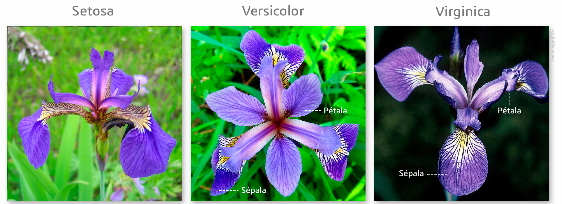
Data frames are rectangular in that they have both rows and columns (unlike vectors), with each column having the same number of rows, the columns are named. Entries within each column must be the same type (if a column has numeric values in it, then they all must be numeric), but different columns are allowed to have different types (numerics, logicals, characters, etc).
There are many datasets that are built into R. These can be accessed using the data() function, as illustrated with the iris dataset above.
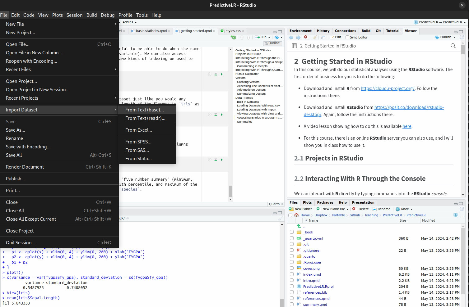
There are several ways to load data frames into R. The simplest way is to import the dataset using RStudio by clicking File -> Import Dataset -> From Text (readr). This will recognize most common data formats; in this course, we will typically have data stored with the .csv extension. After loading the dataset, some code will be given in the bottom-left corner that shows how to load the dataset, and this is useful if you ever want to have the data loaded when running a script without needing to manually import it again. So on my own personal computer I can load the Medical Expenditure Panel Survey (MEPS) from the year 2011 by running the command
library(readr)
meps2011 <- read_csv("~/Dropbox/Portable/Github/Data/MEPS/meps2011.csv")
This will be different on your computer unless you happen to have saved this exact dataset in exactly the same place I did.
Practice this by downloading the dataset satgpa.csv from the following link: https://github.com/theodds/SDS-348/blob/master/satgpa.csv. Put this in some directory on your computer, Then try using read_csv to load it as above by copying its file path.
It is also possible to load a dataset that you have downloaded by using File->Import Dataset->From Text (Base):
For the sake of being able to replicate your work, I strongly suggest you save the commands that RStudio uses to load the data. In addition to appearing in the import menu, they will also appear in the console. You can then save the commands in a script to use again later.
The View() function can be used to take a quick peak at a dataset without printing it:
View(iris)If you run this command, you will be able to scroll through the rows and columns of iris. We can also print the first few rows of the dataset using the head function:
head(iris) Sepal.Length Sepal.Width Petal.Length Petal.Width Species
1 5.1 3.5 1.4 0.2 setosa
2 4.9 3.0 1.4 0.2 setosa
3 4.7 3.2 1.3 0.2 setosa
4 4.6 3.1 1.5 0.2 setosa
5 5.0 3.6 1.4 0.2 setosa
6 5.4 3.9 1.7 0.4 setosaThis is much more manageable than printing the entire dataset.
To access an individual column in an R data frame, we use the $ symbol as in
iris$SpeciesIf you run this command in the console, we will only see at most the first 1000 entries.
Try this and see what happens!
We can use head to see just a few entries instead:
head(iris$Species)[1] setosa setosa setosa setosa setosa setosa
Levels: setosa versicolor virginicaAlternatively, we could also do
head(iris[,"Species"])[1] setosa setosa setosa setosa setosa setosa
Levels: setosa versicolor virginicahead(iris[["Species"]])[1] setosa setosa setosa setosa setosa setosa
Levels: setosa versicolor virginicato get the same effect (using strings in this way to index data frames is useful when the name of the column you want is itself stored in another variables). We can also access different rows of the data frame using the same kinds of indexing we used to index vectors
iris[1:3,"Species"][1] setosa setosa setosa
Levels: setosa versicolor virginicairis$Species[1:3][1] setosa setosa setosa
Levels: setosa versicolor virginicaThe $ symbol lets you treat the columns of the dataset just like you would any vector. For example, we can compute the average sepal length of the flowers in iris as
mean(iris$Sepal.Length)[1] 5.843333We can get a summary of the overall characteristics of each of the columns using the summary function as
summary(iris) Sepal.Length Sepal.Width Petal.Length Petal.Width
Min. :4.300 Min. :2.000 Min. :1.000 Min. :0.100
1st Qu.:5.100 1st Qu.:2.800 1st Qu.:1.600 1st Qu.:0.300
Median :5.800 Median :3.000 Median :4.350 Median :1.300
Mean :5.843 Mean :3.057 Mean :3.758 Mean :1.199
3rd Qu.:6.400 3rd Qu.:3.300 3rd Qu.:5.100 3rd Qu.:1.800
Max. :7.900 Max. :4.400 Max. :6.900 Max. :2.500
Species
setosa :50
versicolor:50
virginica :50
For numeric variables, summary() gives the “five number summary” (minimum, 25th percentile, 50th percentile, average, 75th percentile, and maximum of the column). For character variables (like Species) I find it more useful to examine the column using table():
table(iris$Species)
    setosa versicolor  virginica
        50         50         50
or by making a barplot():
barplot(table(iris$Species))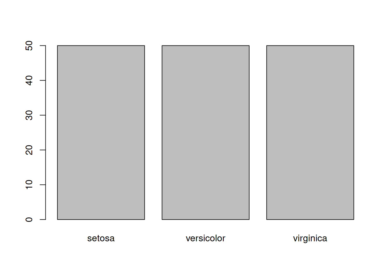
The $ symbol can also be used to add columns to a data frame. For example, we can add the square of Sepal.Length by running
iris$Sepal.Width.Squared <- iris$Sepal.Width^2We can also select a subset of the rows in the data frame using the subset() function
new_iris <- subset(iris, iris$Species == "versicolor")
head(new_iris)
Sepal.Length Sepal.Width Petal.Length Petal.Width Species
51 7.0 3.2 4.7 1.4 versicolor
52 6.4 3.2 4.5 1.5 versicolor
53 6.9 3.1 4.9 1.5 versicolor
54 5.5 2.3 4.0 1.3 versicolor
55 6.5 2.8 4.6 1.5 versicolor
56 5.7 2.8 4.5 1.3 versicolor
Sepal.Width.Squared
51 10.24
52 10.24
53 9.61
54 5.29
55 7.84
56 7.84subset() can also be used to select some of the columns (or remove some of the columns)
## Get flowers with petal length larger than 1.5, retaining only species and
## petal length
head(subset(iris, iris$Sepal.Length > 1.5, select = c(Species, Petal.Length)))
Species Petal.Length
1 setosa 1.4
2 setosa 1.4
3 setosa 1.3
4 setosa 1.5
5 setosa 1.4
6 setosa 1.7## Get flowers with petal length larger than 1.5, removing Species
head(subset(iris, iris$Sepal.Length > 1.5, select = -Species)) Sepal.Length Sepal.Width Petal.Length Petal.Width Sepal.Width.Squared
1 5.1 3.5 1.4 0.2 12.25
2 4.9 3.0 1.4 0.2 9.00
3 4.7 3.2 1.3 0.2 10.24
4 4.6 3.1 1.5 0.2 9.61
5 5.0 3.6 1.4 0.2 12.96
6 5.4 3.9 1.7 0.4 15.21Finally, we can sort the data frame using the order() command. To sort iris according to species and then sepal length, we can do
iris[order(iris$Species, iris$Sepal.Length), ]Run this on your own to see what this does!
We can also do this in decreasing order using a minus sign:
iris[order(iris$Species, -iris$Sepal.Length), ]satgpa.csv dataset that you downloaded at the beginning of this chapter. Use either read.csv or load it by importing it directly.head() and View() functions to look at the dataset. What is inside?data("CO2") to load the built in CO2 dataset. View it, and then run help(CO2) to get more details.summary on satgpa. What does it say about the SAT scores of students in the sample?subset(satgpa, satgpa$sex == 1) do?Visualizations provide an efficient way to display your data to reveal trends and facilitate comparisons. In this course I will mostly introduce visualization tools as required, but I will provide a brief overview of visualization in R here. For a more in-depth treatment of data visualization in R see this free textbook: https://r4ds.had.co.nz/data-visualisation.html. Note that this link uses the ggplot2 framework, which I will not use here because it has a steeper learning curve than just using built-in functions. You can use ggplot2 as an alternative to the plotting functions I discuss here if you are already more comfortable with it.
Scatterplots visualize the relationship between numeric variables, with one of the variables plotted on the x-axis and the other on the y-axis. To create a scatter plot in R we can use the plot() function:
plot(iris$Petal.Length, iris$Petal.Width, main = "Iris Petals",
     xlab = "Petal Length", ylab = "Petal Width")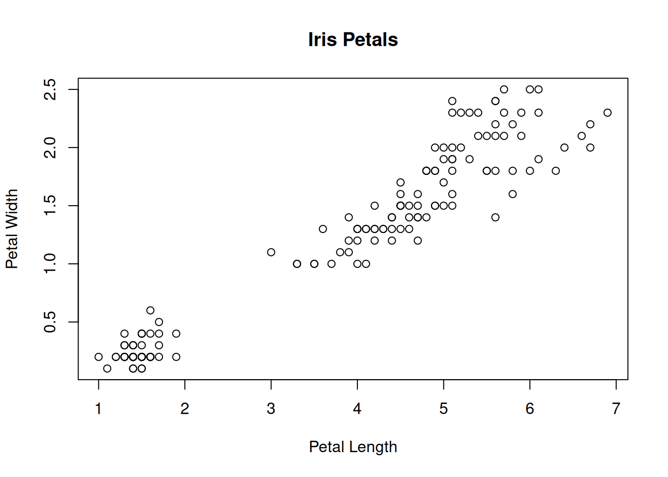
The plot() function takes the following arguments:
x: The variable to display on the x-axisy: The variable to display on the y-axismain: The title of the plot (optional)xlab: The label on the x-axis (optional)ylab: The label on the y-axis (optional)We can add a best-fitting line passing through the data using the lm() and abline() functions:
plot(iris$Petal.Length, iris$Petal.Width, main = "Iris Petals",
     xlab = "Petal Length", ylab = "Petal Width")

petal_lm <- lm(Petal.Width ~ Petal.Length, data = iris)
abline(petal_lm, col = 'skyblue2', lwd = 2)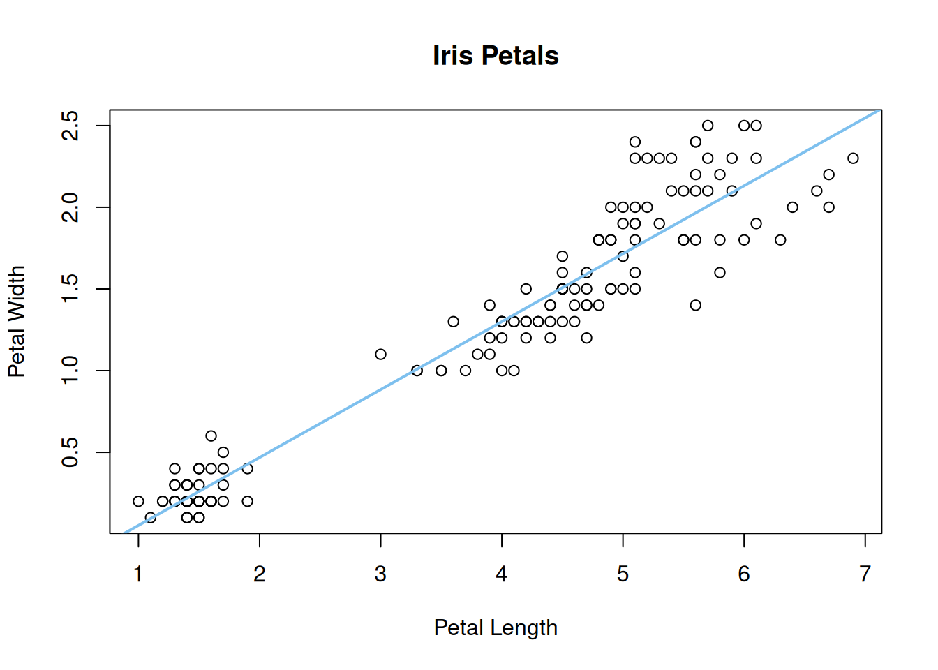
The abline() function takes the following arguments among others:
model: The fitted linear model objectcol: The color of the regression line (optional)lwd: The width the line (optional)More detail later on the lm() function, which fits a linear regression to the data!
We can also customize various features of our plots, such as the point shapes, colors, sizes, etc. using additional arguments in the plot() function:
# Create a customized scatter plot
plot(iris$Petal.Length, iris$Petal.Width, main = "Customized Scatter Plot",
     xlab = "X", ylab = "Y", pch = 3, col = "green", cex = 0.9)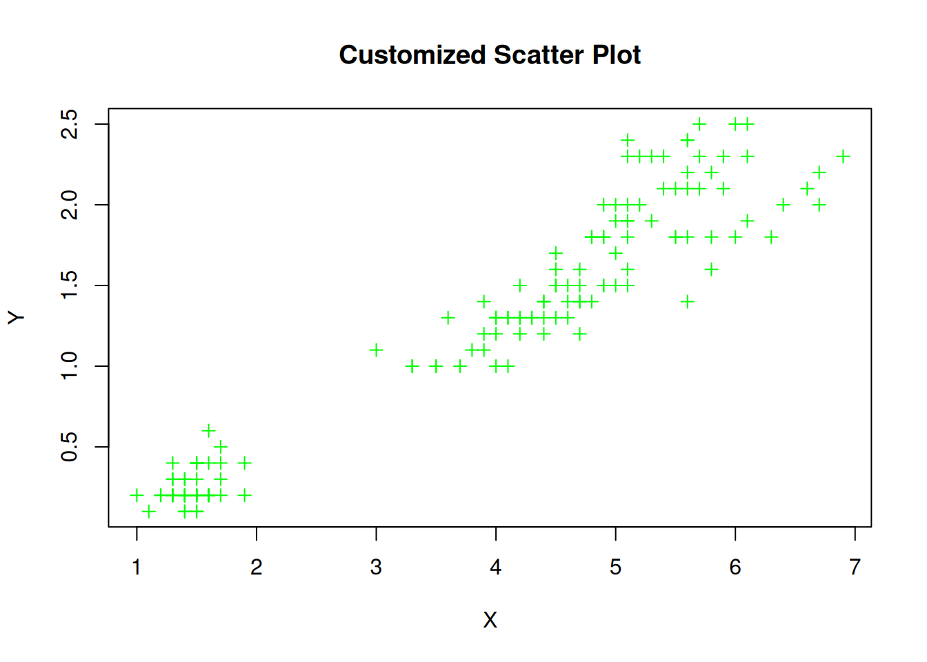
The additional arguments we used are:
pch: The point shape (e.g., 3 for + symbols)col: The color of the pointscex: The size of the pointsDetails on the histogram are given in the next chapter, but for the sake of self containment I reproduce the text here:
The histogram works by (i) dividing up numeric data into bins (in the above case, 0 to 0.5, 0.5 to 1, 1 to 1.5, etc) and then makes a plot with bars where the height of each bar is equal to the number of individuals in that bin. From this, we can see that typical GPAs lie between 2 and 3. There is also a left skew in the data: there is more variability to the left of the typical GPA than to the right.
Code for reproducing the histogram is given below:
fygpa <- read.csv("https://raw.githubusercontent.com/theodds/SDS-348/master/satgpa.csv")
hist(fygpa$fy_gpa)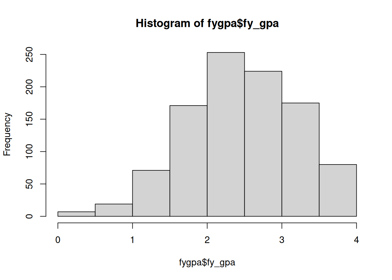
The following code uses optional arguments to make it look a bit nicer:
hist(fygpa$fy_gpa,
     breaks = 20,               # Increase the number of bins
     col = "skyblue",           # Set the color of the bars
     border = "white",          # Set the color of the borders
     main = "Distribution of First-Year GPA",  # Main title
     xlab = "First-Year GPA",   # X-axis label
     ylab = "Frequency",        # Y-axis label
     xlim = c(0, 4),            # Set the x-axis limits
     ylim = c(0, 150),          # Set the y-axis limits
     las = 1,                   # Make y-axis labels horizontal
     cex.main = 1.5,            # Increase the font size of the title
     cex.lab = 1.2,             # Increase the font size of axis labels
     cex.axis = 1)              # Increase the font size of axis values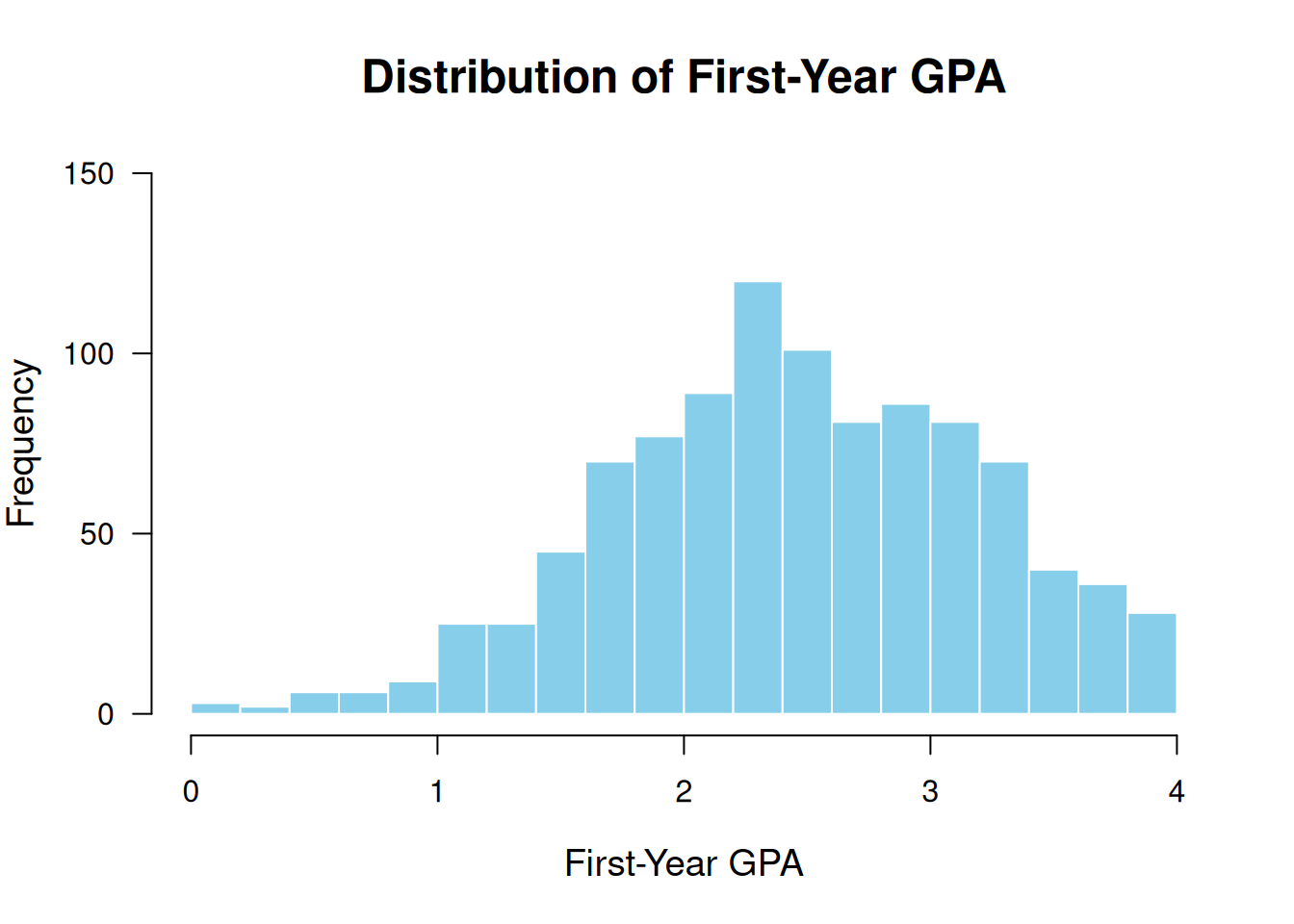
Boxplots are useful when we are interested in visualizing the relationship between a categorical variable and a numeric variable, with the values of the categorical varibale usually on the x-axis and a variety of summaries of the numeric variable (including the median, quartiles, and outliers) on the y-axis. The main components of a box plot are:
Median: The middle value of the dataset, represented by a horizontal line inside the box.
Interquartile Range (IQR): The box itself represents the middle 50% of the data, with the bottom and top edges of the box indicating the first quartile (Q1, 25th percentile) and third quartile (Q3, 75th percentile), respectively.
Whiskers: The vertical lines extending from the box, called whiskers, represent the range of the data outside the IQR. The upper whisker extends to the largest value no further than 1.5 times the IQR from the top of the box, while the lower whisker extends to the smallest value no further than 1.5 times the IQR from the bottom of the box.
Outliers: Points beyond the whiskers are considered outliers and are plotted individually as dots or asterisks.
To create a boxplot we can use the boxplot function:
boxplot(Petal.Length ~ Species, data = iris, main = "Petal Length vs. Species",
        xlab = "Species", ylab = "Petal Length")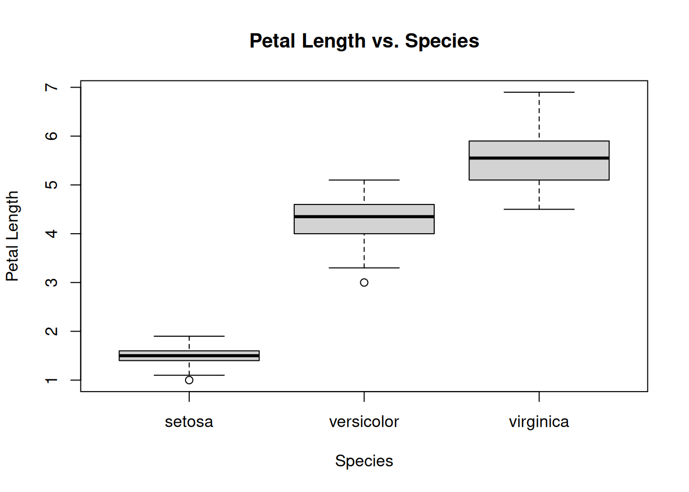
So, for example, we can read from the above boxplot that (i) the median petal length of versicolor’s is around 4.5, (ii) the largest flower has a petal length of around 7, and (iii) 75% of virginica’s have petal lengths less than around 6.
The boxplot() function takes a formula as its main argument, with the numeric variable on the left side of the tilde (~) and the categorical variable on the right side. Additional arguments incldue:
main: The title of the plot (optional)xlab: The label for the x-axis (optional)ylab: The label for the y-axis (optional)mtcars dataset, which you can load by running data('mtcars'). Use help(mtcars) to see what is contained in this dataset.mtcars.mpg across different values of vs.In addition to all of the functions and features built into R, there is a rich ecosystem of additional functionality that the community has built over time. The most common way to share code with the R community is through a package.
To use a package, we first need to have it installed on our computer. To do this, I recommend clicking Install in the Packages frame in RStudio as illustrated below:
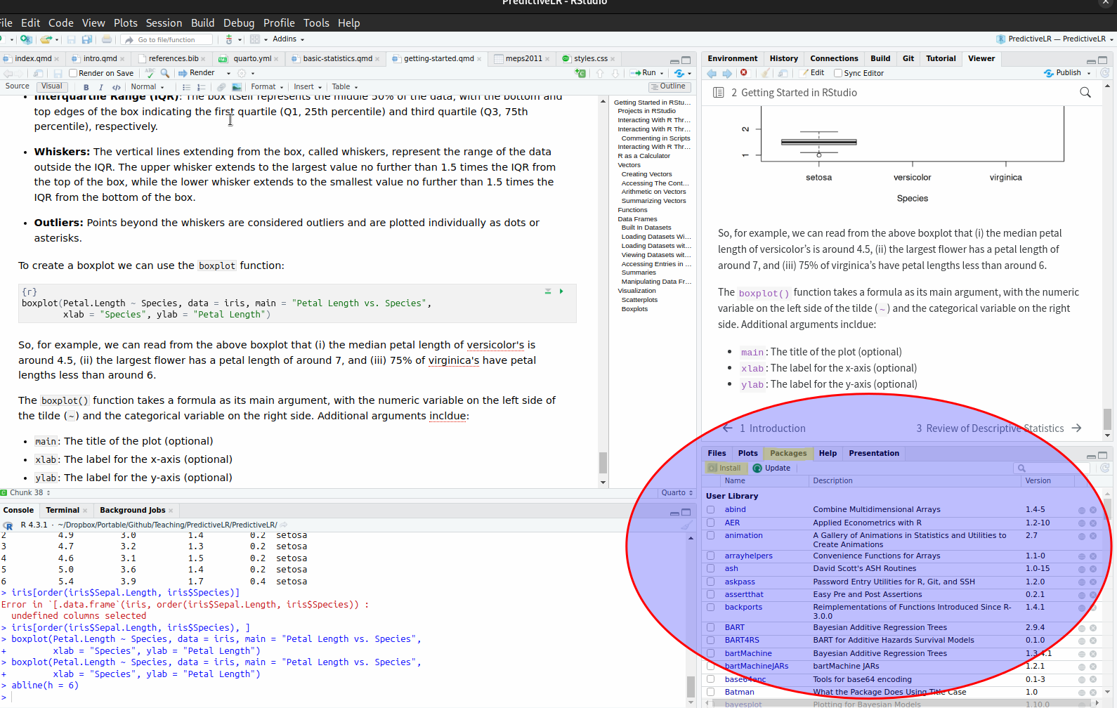
We can then type the name of the package we want to install, in this case the dplyr package. This downloads the package from a repository of packages called CRAN (Comprehensive R Archive Network). This only needs to be done once!
As an alternative to using Packages -> Install, you can use the install.packages() function:
install.packages("dplyr")Do not put install commands in your Quarto documents! Your document won’t render if you do this, and then you will either give up or come to me asking for help. I recommend just avoiding using install.packages(), because you are going to forget I told you not to do this.
After installing a package, we need to load it into our R session to use it. We can do this by running the library() command in our script or in a Quarto document. For example, to load dplyr we can run
library(dplyr)The package dplyr contains a bunch of useful functions for manipulating data frames that were not previously available! For example, we can use the filter() function, which is a slightly-nicer version of the subset() function in base R
filter(iris, Species == "versicolor") Sepal.Length Sepal.Width Petal.Length Petal.Width Species
1 7.0 3.2 4.7 1.4 versicolor
2 6.4 3.2 4.5 1.5 versicolor
3 6.9 3.1 4.9 1.5 versicolor
4 5.5 2.3 4.0 1.3 versicolor
5 6.5 2.8 4.6 1.5 versicolor
6 5.7 2.8 4.5 1.3 versicolor
7 6.3 3.3 4.7 1.6 versicolor
8 4.9 2.4 3.3 1.0 versicolor
9 6.6 2.9 4.6 1.3 versicolor
10 5.2 2.7 3.9 1.4 versicolor
11 5.0 2.0 3.5 1.0 versicolor
12 5.9 3.0 4.2 1.5 versicolor
13 6.0 2.2 4.0 1.0 versicolor
14 6.1 2.9 4.7 1.4 versicolor
15 5.6 2.9 3.6 1.3 versicolor
16 6.7 3.1 4.4 1.4 versicolor
17 5.6 3.0 4.5 1.5 versicolor
18 5.8 2.7 4.1 1.0 versicolor
19 6.2 2.2 4.5 1.5 versicolor
20 5.6 2.5 3.9 1.1 versicolor
21 5.9 3.2 4.8 1.8 versicolor
22 6.1 2.8 4.0 1.3 versicolor
23 6.3 2.5 4.9 1.5 versicolor
24 6.1 2.8 4.7 1.2 versicolor
25 6.4 2.9 4.3 1.3 versicolor
26 6.6 3.0 4.4 1.4 versicolor
27 6.8 2.8 4.8 1.4 versicolor
28 6.7 3.0 5.0 1.7 versicolor
29 6.0 2.9 4.5 1.5 versicolor
30 5.7 2.6 3.5 1.0 versicolor
31 5.5 2.4 3.8 1.1 versicolor
32 5.5 2.4 3.7 1.0 versicolor
33 5.8 2.7 3.9 1.2 versicolor
34 6.0 2.7 5.1 1.6 versicolor
35 5.4 3.0 4.5 1.5 versicolor
36 6.0 3.4 4.5 1.6 versicolor
37 6.7 3.1 4.7 1.5 versicolor
38 6.3 2.3 4.4 1.3 versicolor
39 5.6 3.0 4.1 1.3 versicolor
40 5.5 2.5 4.0 1.3 versicolor
41 5.5 2.6 4.4 1.2 versicolor
42 6.1 3.0 4.6 1.4 versicolor
43 5.8 2.6 4.0 1.2 versicolor
44 5.0 2.3 3.3 1.0 versicolor
45 5.6 2.7 4.2 1.3 versicolor
46 5.7 3.0 4.2 1.2 versicolor
47 5.7 2.9 4.2 1.3 versicolor
48 6.2 2.9 4.3 1.3 versicolor
49 5.1 2.5 3.0 1.1 versicolor
50 5.7 2.8 4.1 1.3 versicolor
Sepal.Width.Squared
1 10.24
2 10.24
3 9.61
4 5.29
5 7.84
6 7.84
7 10.89
8 5.76
9 8.41
10 7.29
11 4.00
12 9.00
13 4.84
14 8.41
15 8.41
16 9.61
17 9.00
18 7.29
19 4.84
20 6.25
21 10.24
22 7.84
23 6.25
24 7.84
25 8.41
26 9.00
27 7.84
28 9.00
29 8.41
30 6.76
31 5.76
32 5.76
33 7.29
34 7.29
35 9.00
36 11.56
37 9.61
38 5.29
39 9.00
40 6.25
41 6.76
42 9.00
43 6.76
44 5.29
45 7.29
46 9.00
47 8.41
48 8.41
49 6.25
50 7.84The point of this section isn’t for your to learn about dplyr. I am just using this package for illustration purposes.
Packages also can have documentation associated to them that can be accessed using the help() function. For example, running
help(dplyr)pulls up the documentation for the dplyr package.