fygpa <- read.csv("https://raw.githubusercontent.com/theodds/SDS-348/master/satgpa.csv")
fygpa$sex <- ifelse(fygpa$sex == 1, "Male", "Female")
fygpa_lm <- lm(fy_gpa ~ hs_gpa, data = fygpa)6 Statistical Inference for Linear Regression
Having reviewed linear regression, we will now discuss performing statistical inference for the slope and intercept in a simple linear regression.
6.1 Running Example: GPAs, Again
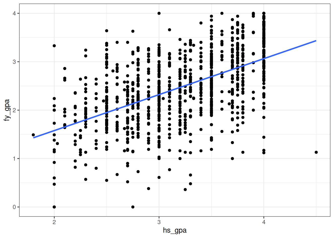
Let’s return to our GPA example, where we treated high school GPA as an independent variable and first year GPA as a dependent variable. The data looked like this:
We will be interested in questions like the following one:
Example: GPAs Again
From our analysis of high school and college GPAs, we found an increasing relationship between high school GPA and first year GPA - students with higher high school GPAs tend to have higher first year GPAs. But this is a statement only about the 1000 students that we happen to have sampled, not about the many more students that could have been sampled in this study but were not. Are we sure, on the basis of the data, that if we had measured the entire population that there would actually be a relationship between these variables? If so, what lines would we plausibly get if we ran a linear regression on the entire population?
In the above example, we might think of the population as consisting of either all students at the school or, more interestingly, all hypothetical students that could have been admitted in the past or will be admitted in the future.
6.2 Working Assumptions
The standard way of teaching inference for linear regression is to introduce a bunch of assumptions about how the data was generated and then show how to do statistical inference when these assumptions are satisfied. Despite not really being correct, these working assumptions are often close enough to be correct that they can be a useful starting point for understanding what a linear regression is doing. Towards the end of this chapter we will discuss what occurs when the assumptions are not true.
In rough order of importance, these assumptions are as follows.
Assumptions for Simple Linear Regression
Let \((X_1, Y_1), \ldots, (X_N, Y_N)\) be a collection of independent variables \((X_i)\) and dependent variables \((Y_i)\).
Working Assumption 0 (“Full Rank”): Not all of the \(X_i\)’s are equal to each other.
Working Assumption 1 (Linearity): We can write \(Y_i = \beta_0 + \beta_1 \, X_i + \epsilon_i\) for some intercept \(\beta_0\), slope \(\beta_1\), and error term \(\epsilon_i\). Additionally, we assume population average of the \(\epsilon_i\)’s is \(0\).
Working Assumption 2 (Uncorrelated errors): The \(\epsilon_i\)’s are uncorrelated with each other.
Working Assumption 3 (Constant Error Variance): The variance of the \(\epsilon_i\)’s is the same for all \(i\); we let \(\sigma^2\) be this common variance.
Working Assumption 4 (Normality): The \(\epsilon_i\)’s are independent of each other and have a normal distribution, given \(X_1, \ldots, X_N\).
The \(X\)’s Are Treated as Fixed
Under the assumptions listed above, we typically proceed as though the \(X_i\)’s were non-random. So, we treat the independent variable \(X_i\) as though it were not random, but \(Y_i\) as though it were. Recall that what it means for us for something to “be random” is that if you replicated your experiment/survey/whatever then you would get different values, so in the case of something like the GPA dataset you would probably get different high school GPAs if you reran the study (and so the \(X_i\)’s would not be fixed).
We are doing this mainly because (i) treating the \(X_i\)’s as fixed makes the math a little bit easier to explain, (ii) because sometimes (as in experimental settings) the \(X_i\)’s actually are known, and (iii) because treating the \(X_i\)’s as fixed when they are actually random does not actually change any of the methods we are going to use.
We now discuss each of the assumptions in detail.
6.2.1 The “Full Rank” Assumption
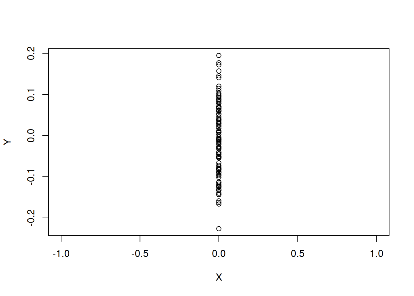
This assumption just says that the independent variable has more than one value in the sample; it is not really much of an assumption, and is virtually always satisfied in practice. This makes sense, as it would be difficult to fit a linear to data that looks like this:
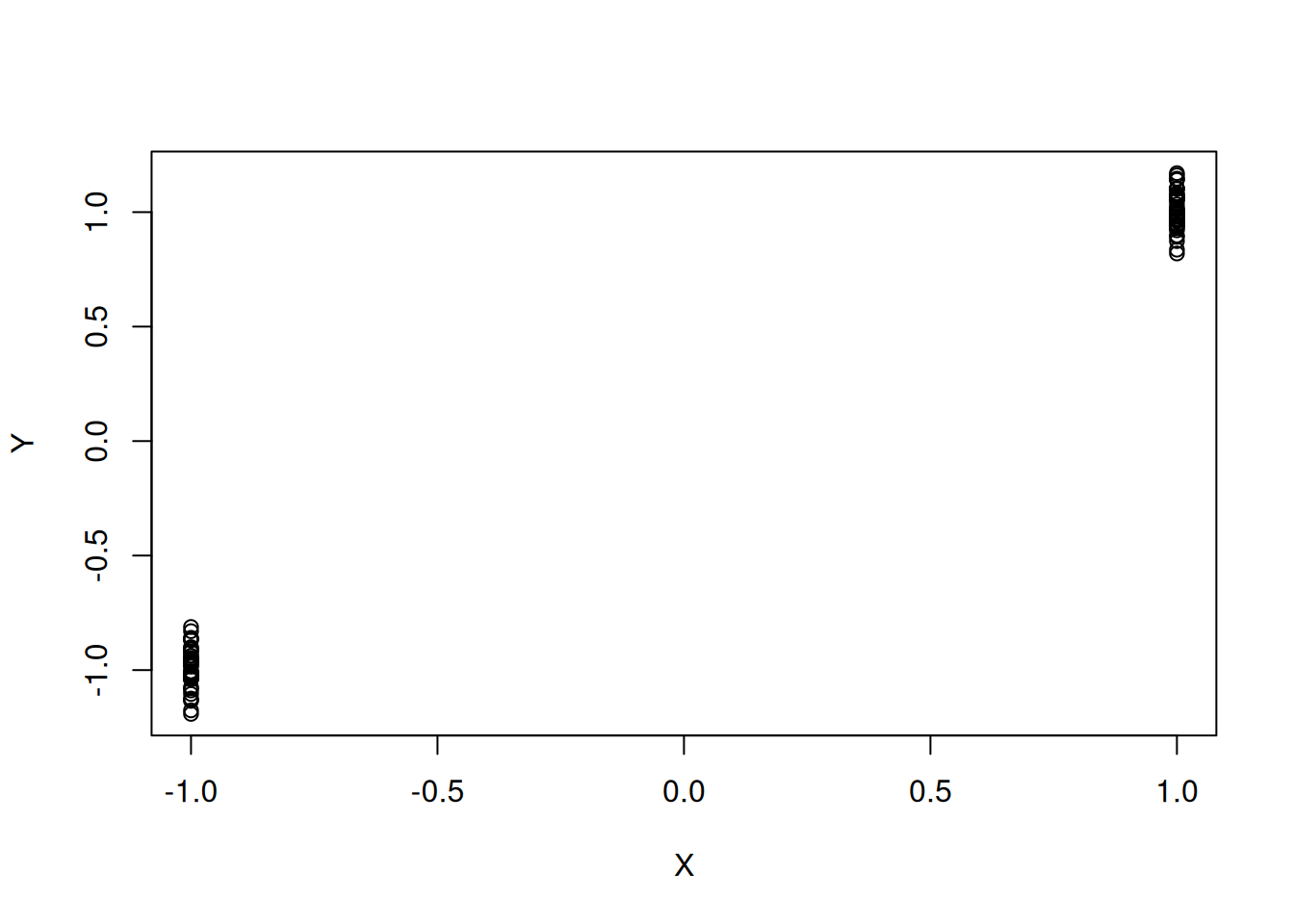
On the other hand, if we had even just one more unique value of \(X_i\) we could make progress:
This assumption is not very stringent (which is why it is listed as Assumption 0 rather than Assumption 1), but interestingly we will see that a version of this assumption becomes important when we start controlling for multiple independent variables rather than a single independent variable.
6.2.2 The Linearity Assumption
The linearity assumption states that
\[ Y_i = \beta_0 + \beta_1 \, X_i + \epsilon_i \]
for some slope \(\beta_1\) and intercept \(\beta_0\), with \(E(\epsilon_i) = 0\). Another way of saying this is that the population average value of \(Y_i\) is \(E(Y_i) = \beta_0 + \beta_1 \, X_i\), so that it is linear in \(X_i\). For the GPA dataset it looks plausible because, while the points do not fall directly on the line, it does look like the average for each value of high school GPA might be on the line:
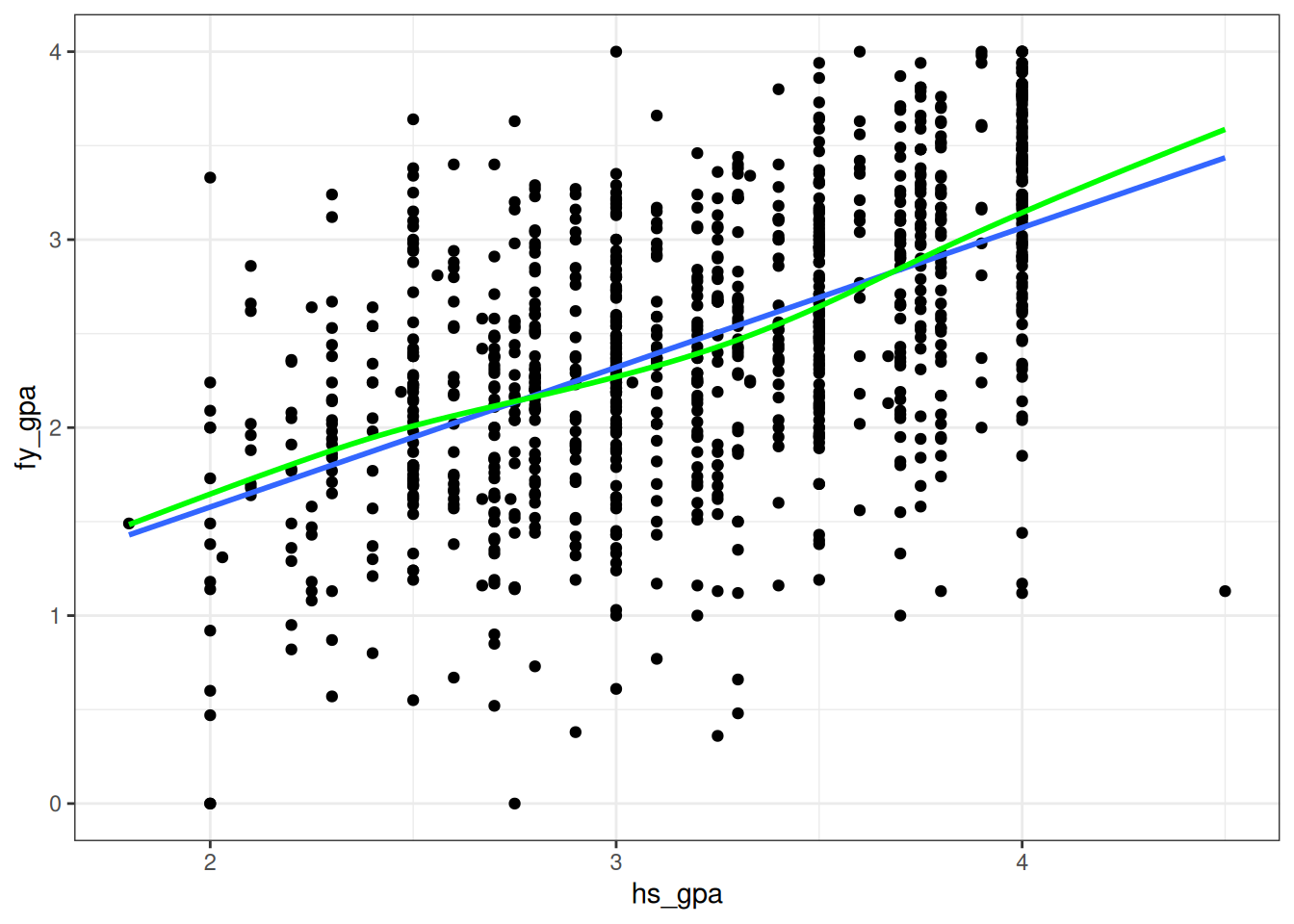
In the above figure, I have superimposed both the fit of the linear regression and the fit of a different method which does not make the linearity assumption (i.e., it allows the relationship between high school and first year GPA to be curved), and we see that the two methods more-or-less agree. This is not the case for the following dataset:

The above displays the relationship between temperature on a given day in a US city and the electricity usage in that city (we’ll discuss this dataset in more detail later). The main point we want to make here is just that the relationship between these variables is non-linear: electricity usage decreases as the temperature increases, but the relationship is clearly curved as we get to higher temperatures. The least squares fit is given by the blue line, while a more advanced non-linear fit is given in green.
When Is This Assumption True?
I am of the opinion that this assumption is rarely true, and if it is true it is probably because there is a good subject-matter reason to expect it to be true. I do not think the relationship in either of the two above examples is “really” linear.
That does not mean it is useless to use as a working assumption, as there are a lot of datasets where the assumption is “almost true” - things are close enough to linear that you can get away with just assuming things are linear and reality will not punish you if you are wrong. The GPA dataset is like this: even though the relationship probably isn’t really linear (especially if we extended to very low GPAs) it is unlikely that we will be misled if you just proceed as though it were. Later in this course we will discuss actually checking these assumptions in detail!
6.2.4 The Constant Error Variance Assumption
The constant error variance assumption, also known as homoscedasticity, states that the variance of the errors \(\epsilon_i\) is constant for all values of the independent variable \(X_i\). In other words, the spread of the \(Y_i\) values around the true regression line \(\beta_0 + \beta_1 X_i\) is the same for all values of \(X_i\).
Mathematically, this assumption can be written as:
\[ \text{Var}(\epsilon_i) = \sigma^2 \text{ for all } i \]
where \(\sigma^2\) is a constant.
When this assumption is violated, we say that the errors are heteroscedastic. Heteroscedasticity can occur when the variability of \(Y_i\) changes systematically with the value of \(X_i\). Heteroscedasticity is fairly common:
When \(Y_i\) represents a count (e.g., number of movies you have watched in the past year, number of pets you have, number of earthquakes in a given area) we usually expect a large predicted count to also be associated with larger variability. For example, the number of earthquakes in Austin in a given year is close to zero, with a variance that is also close to zero; on the other hand, the number of noticeable earthquakes in LA is larger, with roughly five earthquakes per year in the 3.0 - 4.0 magnitude range, and with the variance of the number of earthquakes also in this range.
Income and expenditure data also tends to be heteroscedastic - people with high predicted incomes also have high variability in their incomes. A famous actor, for example, might have a yearly income that swings by millions of dollars year-over-year, while a college professor might have an income that varies by a couple tens-of-thousands.
What If This Assumption is Wrong?
Violations of the constant variance assumption, like the correlated errors assumption, tend to affect the precision of the estimates rather than their accuracy, and cause the formulas for the standard errors of \(\widehat\beta_0\) and \(\widehat\beta_1\) we give below to be incorrect.
6.2.5 The Normality Assumption
The final working assumption is that the errors \(\epsilon_i\) in the model \(Y_i = \beta_0 + \beta_1 \, X_i + \epsilon_i\) follow a normal distribution; in combination with Assumption 1 (Linearity) and Assumption 3 (Constant Error Variance) it follows that
\[ \epsilon_i \text{ has a normal distribution with mean } 0 \text{ and variance } \sigma^2. \]
The following figure gives a visual representation of what this means:
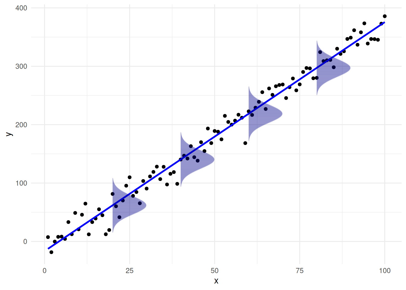
Basically this assumption implies that, for any fixed value of \(X_i\), the corresponding \(Y_i\) values are normally distributed around the true regression line \(\beta_0 + \beta_1 \, X_i\) with the same variance \(\sigma^2\) for all values of \(X_i\); about each point on the line above, the vertical deviations from the line follow a normal distribution. By contrast, this assumption is not satisfied for the following dataset:
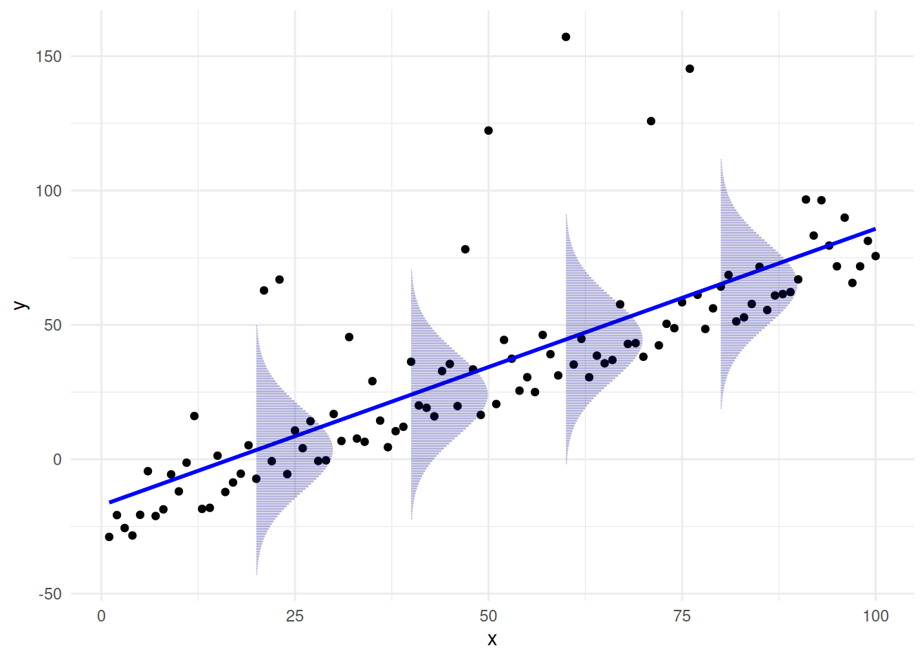
In the above plot, we can see that the results are not normally distributed about the line because the errors are not symmetric about the line: there are many errors below the line, which are canceled out by a few large errors above the line. Note that, in this example, all of the other assumptions are actually satisfied: the population average of the \(\epsilon_i\)’s is zero, the \(\epsilon_i\)’s are uncorrelated, and the variance is constant. The only problem is that the errors are not normally distributed.
One quick way to check whether the errors are normally distributed or not is to look at a histogram of the residuals and see if it looks close to a normal distribution. For the previous two plots, this is what a histogram of the residuals looks like:
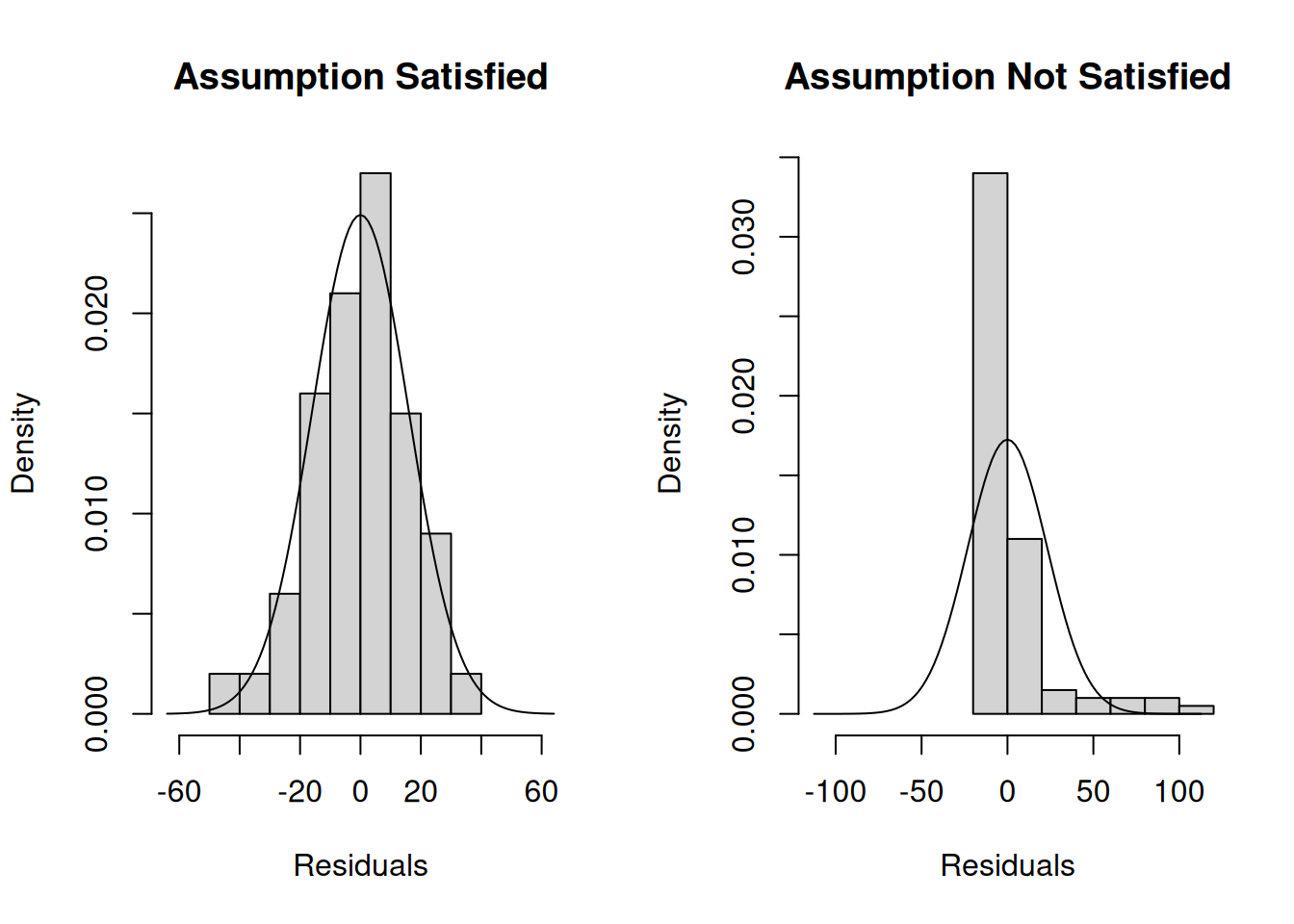
We see that when the assumptions are satisfied the residuals follow roughly a bell-shaped curve, while when the assumptions are not satisfied they do not. For comparison, the density of the normal distribution is also displayed.
For the GPA dataset, the residuals look like this:
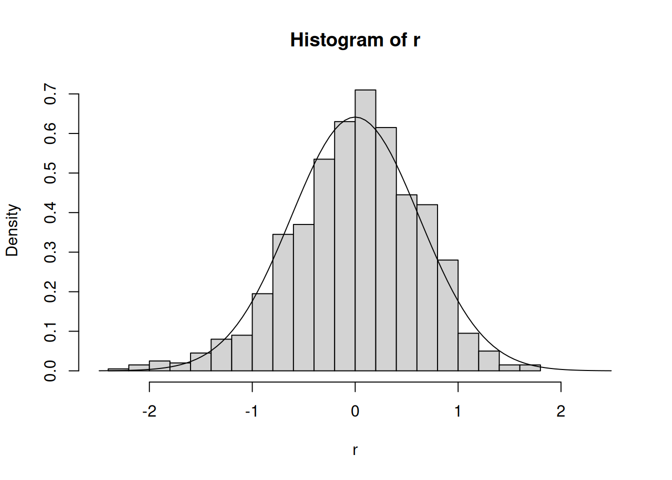
This seems pretty good, although it seems like there might be a few more very-negative residuals than very-positive residuals. In the chapter on diagnostics, we will look at checking this assumption in more detail.
What If This Assumption Is Not True?
This assumption is usually untrue, and unlike the other assumptions it is often pretty easy to show it is not true. It is also the least important assumption to get correct. The consequence of this assumption being wrong is that we will instead need to rely on large samples and the central limit theorem when drawing conclusions about \(\beta_0\) and \(\beta_1\); this isn’t so bad, since the central limit theorem will hold unless the sample sizes are very small.
The one case where the normality assumption actually matters a great deal is when we are constructing prediction intervals, which we will discuss later in this chapter. In that case, the normality assumption is critical.
6.3 Properties of \(\widehat \beta_0\) and \(\widehat \beta_1\) Under the Working Assumptions.
When our working assumptions hold, the least squares estimators \(\widehat \beta_0\) and \(\widehat\beta_1\) have many desirable properties. First, the estimators are unbiased: averaged over many replications of your data collection process, you will get the correct answer. The only requirement for this to be the case is that the linearity assumption \(Y_i = \beta_0 + \beta_1 \, X_i + \epsilon_i\) holds where \(E(\epsilon_i) = 0\) for all \(i\); the errors can be correlated, have non-constant variance, or not be normally distributed.
Unbiasedness
Under the full rank and linearity assumptions (Working Assumptions 0 and 1), the least squares estimators \(\widehat \beta_0\) and \(\widehat \beta_1\) are unbiased; in other words, \(E(\widehat \beta_0) = \beta_0\) and \(E(\widehat \beta_1) = \beta_1\).
Unbiasedness basically says that the least squares estimators are accurate. A natural follow up question is: are the least squares estimators precise? For us to be able to say whether they are precise or not requires Working Assumption 2 and Working Assumption 3.
Variance Formula for Slope
Under the full rank, linearity, uncorrelated-errors, and constant-variance assumptions (Working Assumptions 0, 1, 2, and 3), the least squares estimator of the slope \(\widehat \beta_1\) has variance given by
\[ \sigma^2_{\widehat{\beta}_1} = \frac{\sigma^2}{SS_{XX}} = \frac{\sigma^2}{\sum_{i = 1}^N (X_i - \bar X)^2}. \]
The standard error of \(\widehat \beta_1\) is therefore given by
\[ s_{\widehat{\beta}_1} = \frac{s}{\sqrt{SS_{XX}}}. \]
where \(s = \sqrt{\sum_i e_i^2 / (N - 2)}\) is the residual standard error.
Variance Formula for Intercept
Under Working Assumptions 0, 1, 2, and 3, the least squares estimator of the intercept \(\widehat \beta_0\) has variance given by
\[ \sigma^2_{\widehat{\beta}_0} = \sigma^2 \left[\frac{1}{N} + \frac{\bar X^2}{SS_{XX}}\right] = \sigma^2 \left[\frac{1}{N} + \frac{\bar X^2}{\sum_{i = 1}^N (X_i - \bar X)^2} \right]. \]
The standard error of \(\widehat \beta_0\) is therefore given by
\[ s_{\widehat{\beta}_0} = s \sqrt{\frac{1}{N} + \frac{\bar X^2}{SS_{XX}}}, \]
where \(s = \sqrt{\sum_{i=1}^N e_i^2 / (N - 2)}\) is the residual standard error.
So both \(\widehat\beta_0\) and \(\widehat\beta_1\) both become more precise as \(N\) increases. That is reassuring: larger sample sizes lead to more precise estimates of the slope and intercept.
Statistical inference can be based on the standardized versions of \(\widehat\beta_0\) and \(\widehat \beta_1\), which we get by subtracting their average and dividing by their standard error:
\[ T_{\widehat\beta} = \frac{\widehat \beta - \beta}{s_{\widehat\beta}}. \]
If the sample size is large, then \(T_{\widehat \beta}\) will have a standard normal distribution; alternatively, if we add in Working Assumption 4 (normality of the error), then we can give the exact distribution.
Large Sample Distribution of Least Squares
Under Working Assumptions 0, 1, 2, and 3, and some other technical assumptions that we will not go into, the quantity
\[ T_{\widehat\beta} = \frac{\widehat \beta - \beta}{s_{\widehat \beta}} \]
has a probability distribution that is approximately a standard normal distribution (here, \(\widehat \beta\) can be either the slope or the intercept).
If we add in Working Assumption 4, then \(T_{\widehat\beta}\) has exactly a \(t\)-distribution with \(N - 2\) degrees of freedom.
6.4 Inference for the Slope \(\beta_1\)
For simple linear regression, we are usually interested in performing inference about \(\beta_1\) first and foremost; this is because it quantifies the actual relationship between the independent and dependent variables, which is often the primary question of interest in many research contexts. For example, if we find that \(\beta_1 = 0\) then we will be able to conclude that there is no linear relationship between \(X\) (say, high school GPA) and \(Y\) (say, first year GPA), which would be a useful finding. By contrast, while \(\beta_0\) is also an important component of the model, it is often of less scientific relevance than \(\beta_1\); in the GPA example, \(\beta_0\) corresponds to the average first year GPA of a student who had a 0 GPA in high-school, which corresponds to a GPA that we do not even see in the sample. Accordingly, we will begin by performing inference for \(\beta_1\).
Assuming that the working assumptions are true, we perform hypothesis tests and make confidence intervals for the slope. These inference procedures are based on the fact that the \(T\)-statistic \(T_{\widehat\beta_1} = \frac{\widehat\beta_1 - \beta_1}{s_{\widehat\beta_1}}\) has a \(t\)-distribution with \(N - 2\) degrees of freedom (under all of the working assumptions).
6.4.1 Inference in R
The relevant quantities for computing the standard error and \(T\)-statistic for the slope are given in the output of summary here, under the columns Std. Error and t value, respectively, in the coefficients table:
summary(fygpa_lm)
Call:
lm(formula = fy_gpa ~ hs_gpa, data = fygpa)

Residuals:
     Min       1Q   Median       3Q      Max
-2.30544 -0.37417  0.03936  0.41912  1.75240

Coefficients:
            Estimate Std. Error t value Pr(>|t|)
(Intercept)  0.09132    0.11789   0.775    0.439
hs_gpa       0.74314    0.03635  20.447   <2e-16 ***
---
Signif. codes:  0 '***' 0.001 '**' 0.01 '*' 0.05 '.' 0.1 ' ' 1

Residual standard error: 0.6222 on 998 degrees of freedom
Multiple R-squared:  0.2952,    Adjusted R-squared:  0.2945
F-statistic: 418.1 on 1 and 998 DF,  p-value: < 2.2e-16
Using tidy() produces the coefficients table without any of the additional material provided in the output of summary()
tidy(fygpa_lm)# A tibble: 2 × 5
term estimate std.error statistic p.value
<chr> <dbl> <dbl> <dbl> <dbl>
1 (Intercept) 0.0913 0.118 0.775 4.39e- 1
2 hs_gpa 0.743 0.0363 20.4 6.93e-78As a sanity check, we can compute each of the entries in the table for hs_gpa by hand using our formulas:
SSXX <- sum((fygpa$hs_gpa - mean(fygpa$hs_gpa))^2)
SSXY <- sum((fygpa$hs_gpa - mean(fygpa$hs_gpa)) *
              (fygpa$fy_gpa - mean(fygpa$fy_gpa)))

beta_1_hat <- SSXY / SSXX
s <- sigma(fygpa_lm)
s_beta_1_hat <- s / sqrt(SSXX)
t_stat <- beta_1_hat / s_beta_1_hat
p_value <- 2 * pt(q = t_stat, df = 998, lower.tail = FALSE)

c(estimate = beta_1_hat, std.error = s_beta_1_hat, statistic = t_stat,
  p.value = p_value)
estimate std.error statistic p.value
7.431385e-01 3.634501e-02 2.044678e+01 6.932446e-78 In practice you should of course use the output of summary() rather than doing these things by hand.
6.4.2 Hypothesis Testing for the GPA Data
We typically start with the following null and alternative hypotheses:
- \(H_0\): \(\beta_1 = 0\) (there is no linear relationship between \(X\) and \(Y\)).
- \(H_1\): \(\beta_1 \ne 0\) (there is some linear relationship between \(X\) and \(Y\), but it might be positive or negative).
We can then use the \(T\)-statistic to test this hypothesis. Under the null hypothesis (\(\beta_1 = 0\)) we know that \(T = \frac{\widehat\beta_1}{s_{\widehat\beta_1}}\) has a \(t\)-distribution with \(N - 2 = 998\) degrees of freedom. For the two-sided test, which only states that \(\beta\) is different from \(0\), the P-value corresponds to the values of \(T\) more extreme than those that we observed, which are the areas underneath the curve to the left and right of the two cutoffs:
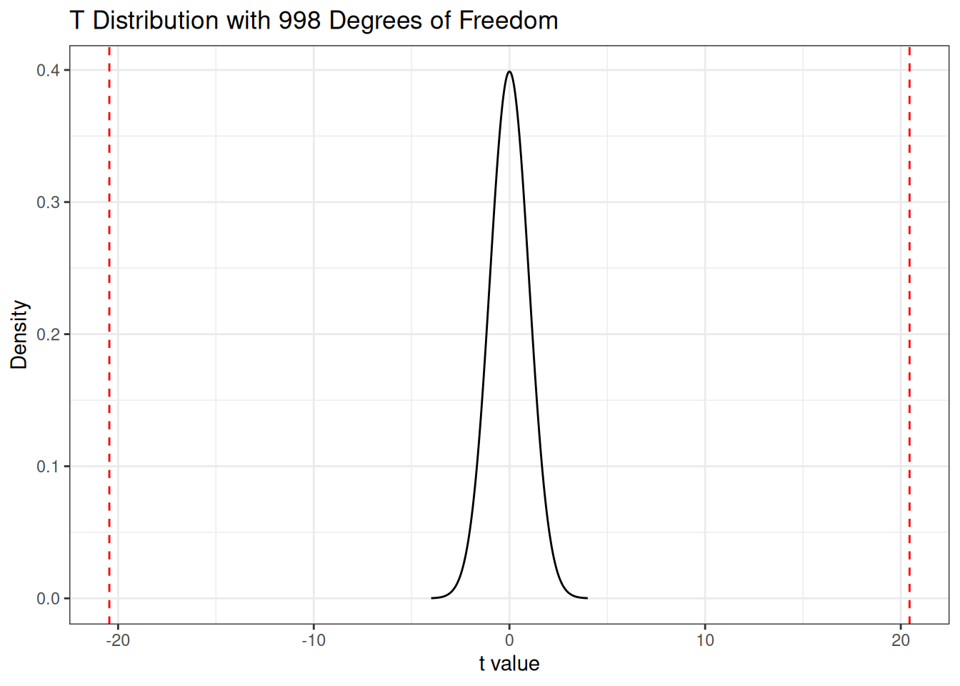
Note that, in this case, the value of \(T\) is so extreme that the areas are basically zero, so the \(P\)-value is \(7 \times 10^{-78}\) (a very significant result).
Very Small \(P\)-Values
The \(P\)-value here is so small that we can safely conclude that \(\beta_1 \ne 0\), i.e., high school GPA and first-year GPA have some association with each other. Actually, however, a \(P\)-value of \(10^{-78}\) is so small that you probably shouldn’t take the precision of this result seriously; we know that the data is not actually normal in reality, and while the sample size is large the normal approximation is not going to be accurate to 78 decimal places. Nevertheless, the \(P\)-value is so small that there really is not much statistics to do here.
6.4.3 Confidence Interval for GPA Data
We can get a confidence interval for \(\beta_1\) using our formula for the standard error as
\[ \beta_1 = \widehat \beta_1 \pm t_{\alpha/2} \times \frac{s}{\sqrt{SS_{XX}}}. \]
Doing this by hand in R we can get a 95% confidence interval by doing the following:
 ## The error rate
alpha <- 0.05

## Get t(alpha / 2) using the qt function
t_cutoff <- qt(p = alpha / 2, df = 998, lower.tail = FALSE)

## Upper and lower intervals
lower <- beta_1_hat - t_cutoff * s_beta_1_hat
upper <- beta_1_hat + t_cutoff * s_beta_1_hat

## Print the result
print(c(lower, upper))
[1] 0.6718171 0.8144599Instead of doing this, we can also use the confint function to make R construct the confidence interval for us:
confint(fygpa_lm) 2.5 % 97.5 %
(Intercept) -0.1400191 0.3226569
hs_gpa 0.6718171 0.8144599Interpretation: We are 95% confident that the true slope is between 0.6718 and 0.8145. What this means is that we are 95% confident that students with a high school GPA of \(x + 1\) have, on average, between 0.6718 and 0.8144 higher first year GPAs than students who have a high school GPA of only \(x\); for example, the population of students with a high school GPA of \(4\) will have between 0.6718 and 0.8144 higher first year GPAs than students with a high school GPA of 3.
6.5 Inference for the Intercept
While we usually do not care about the intercept \(\beta_0\), there are certain occasions where we actually do. Because the intercept is not of interest in the GPA data, we will temporarily change to a different data example where there is interest in both the slope and the intercept.
Example: The following dataset is taken from the textbook Bayesian Data Analysis, 3rd Edition by Gelman et al.1 Gelman describes the dataset as follows:
Football experts provide a point spread for every football game as a measure of the difference in ability between the two teams. For example, team A might be a 3.5-point favorite to defeat team B. The implication of this point spread is that the proposition that team A, the favorite, defeats team B, the underdog, by 4 or more points is considered a fair bet; in other words, the probability that A wins by more than 3.5 points is 1/2. If the point spread is an integer, then the implication is that team A is as likely to win by more points than the point spread as it is to win by fewer points than the point spread (or to lose); there is positive probability that A will win by exactly the point spread, in which case neither side is paid off.
… Each point in the scatterplot displays the point spread, x, and the actual outcome (favorite’s score minus underdog’s score), y. (In games with a point spread of zero, the labels ‘favorite’ and ‘underdog’ were assigned at random.) A small random jitter is added to the x and y coordinate of each point on the graph so that multiple points do not fall exactly on top of each other
The data can be loaded by running
spread <- read.table("https://raw.githubusercontent.com/theodds/StatModelingNotes/master/datasets/spread", header = TRUE)
spread$outcome <- spread$favorite - spread$underdog
head(spread)
home favorite underdog spread favorite.name underdog.name week outcome
1 1 21 13 2.0 TB MIN 1 8
2 1 27 0 9.5 ATL NO 1 27
3 1 31 0 4.0 BUF NYJ 1 31
4 1 9 16 4.0 CHI GB 1 -7
5 1 27 21 4.5 CIN SEA 1 6
6 0 26 10 2.0 DAL WAS 1 16and we can visualize the dataset as
plot(spread$spread, spread$outcome,
     pch = 20, cex = 0.5,
     xlab = "Spread",
     ylab = "Outcome")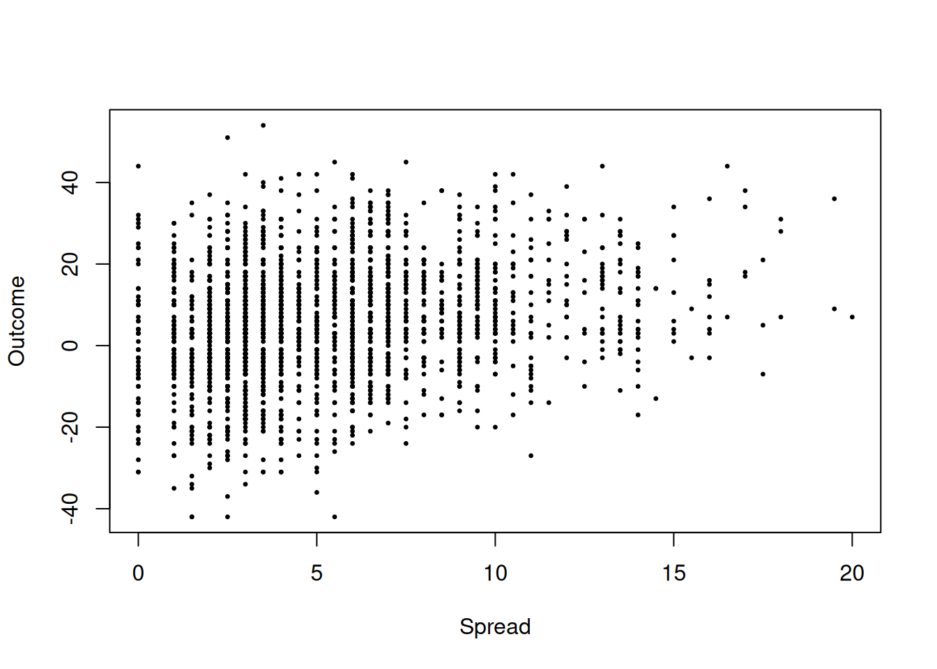
Question: are the experts who set the spread, on average, correct? If we let \(Y_i\) denote the outcome and \(X_i\) the spread that the experts set, then what it would mean for the “experts to be correct on average” would be for \(E(Y_i) = X_i\), i.e., the population average of the outcome of a given game is equal to the spread. But notice that we can rewrite this as
\[ Y_i = \beta_0 + \beta_1 \, X_i + \epsilon_i \qquad \text{where} \qquad \beta_0 = 0, \beta_1 = 1. \]
So, the experts being “right on average” actually corresponds to a very precise claim about both the slope and the intercept! As a quick sanity check, we can see if the line \(y = x\) appears to match the data well:
plot(spread$spread, spread$outcome,
     pch = 20, cex = 0.5,
     xlab = "Spread",
     ylab = "Outcome")

## This adds a linear with intercept 0 and slope 1
abline(a = 0, b = 1)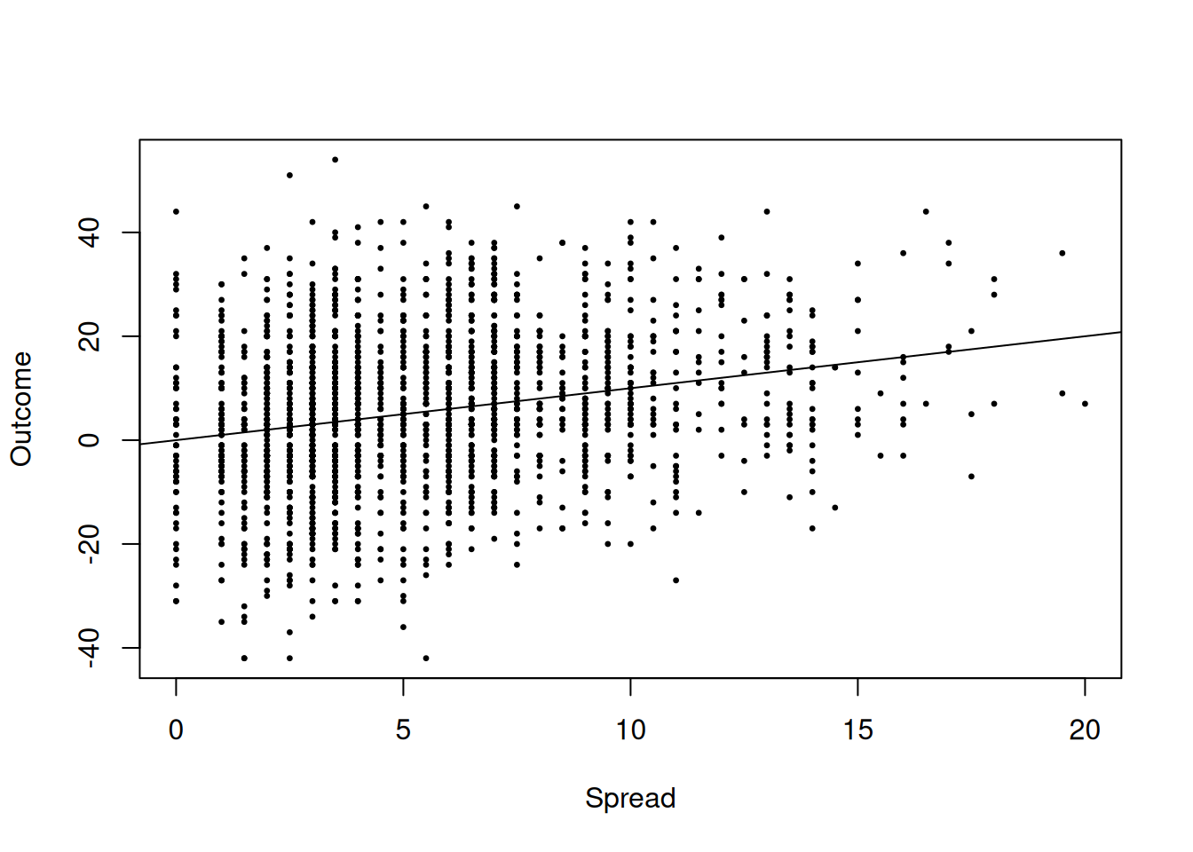
Looks pretty good to me, but to say more we need to do some actual statistical inference.
6.5.1 Hypothesis Testing for the Intercept
Focusing just on the intercept for the spread dataset, we can consider the following null and alternative hypotheses:
- \(H_0\): \(\beta_0 = 0\) (the average outcome of games with an expert spread of zero is also zero).
- \(H_1\): \(\beta_0 \ne 0\) (the average outcome of games with an expert spread of zero is not zero).
Under the null hypothesis, the relevant \(T\)-statistic is
\[ T = \frac{\widehat \beta_0}{s_{\widehat\beta_0}} \qquad \text{where} \qquad \widehat\beta_0 = \bar Y - \widehat\beta_1 \, \bar X \qquad \text{and} \qquad s_{\widehat\beta_0} = s \sqrt{\frac{1}{N} + \frac{\bar X^2}{SS_{XX}}} \]
The test statistic for this test, and the associated \(P\)-value, is given in the coefficients table of summary() under the row intercept:
lm_spread <- lm(outcome ~ spread, data = spread)
summary(lm_spread)
Call:
lm(formula = outcome ~ spread, data = spread)

Residuals:
    Min      1Q  Median      3Q     Max
-47.729  -8.198  -0.222   8.833  50.299

Coefficients:
            Estimate Std. Error t value Pr(>|t|)
(Intercept)  0.15285    0.53000   0.288    0.773
spread       1.01390    0.08449  12.000   <2e-16 ***
---
Signif. codes:  0 '***' 0.001 '**' 0.01 '*' 0.05 '.' 0.1 ' ' 1

Residual standard error: 13.69 on 2238 degrees of freedom
Multiple R-squared:  0.06046,   Adjusted R-squared:  0.06004
F-statistic:   144 on 1 and 2238 DF,  p-value: < 2.2e-16
or using tidy() under the row for intercept:
tidy(lm_spread)# A tibble: 2 × 5
term estimate std.error statistic p.value
<chr> <dbl> <dbl> <dbl> <dbl>
1 (Intercept) 0.153 0.530 0.288 7.73e- 1
2 spread 1.01 0.0845 12.0 3.37e-32From the above, we see that \(\widehat\beta_0 \approx 0.15\), \(s_{\widehat\beta_0} \approx 0.53\), \(T_{\widehat\beta_0} \approx 0.29\), and a \(P\)-value of \(0.77\) for the test above. Based on these results, there is no evidence in the data to disprove the null hypothesis that \(\beta_0\) is equal to zero.
In practice, we of course should use the output of functions like summary() or tidy(). But for the sake of completeness, we will verify the formulas above and show that they lead to the same answers.
X <- spread$spread
Y <- spread$outcome
Xbar <- mean(X)
Ybar <- mean(Y)
N <- length(Y)

SSXX <- sum((X - Xbar)^2)
SSXY <- sum((X - Xbar) * (Y - Ybar))

beta_1_hat <- SSXY / SSXX
beta_0_hat <- Ybar - beta_1_hat * Xbar
s <- sqrt(sum((Y - beta_0_hat - beta_1_hat * X)^2 / (N - 2)))

s_beta_0_hat <- s * sqrt(1 / N + Xbar^2 / SSXX)
t_stat <- beta_0_hat / s_beta_0_hat
p_value <- 2 * pt(t_stat, N - 2, lower.tail = FALSE)

print(c(estimate = beta_0_hat, std.error = s_beta_0_hat, statistic = t_stat,
      p.value = p_value))
estimate std.error statistic p.value
0.1528452 0.5299971 0.2883887 0.7730759 We see that the results agree with the results from tidy() and summary().
6.5.2 Confidence Interval for the Intercept
A confidence interval for the intercept can similarly be constructed as
\[ \beta_0 = \widehat\beta_0 \pm t_{\alpha/2} \times s_{\widehat\beta_0}. \]
We can get a 95% confidence interval for the intercept just as we did for the slope:
alpha <- 0.05
t_alpha_2 <- qt(p = alpha / 2, df = N - 2, lower.tail = FALSE)
lower <- beta_0_hat - t_alpha_2 * s_beta_0_hat
upper <- beta_0_hat + t_alpha_2 * s_beta_0_hat

print(c(lower = lower, upper = upper))
lower upper
-0.8864921 1.1921825 So we are 95% confident that the true intercept is between -0.89 and 1.19. We can also get this directly from the fitted model using the confint() function:
confint(lm_spread) 2.5 % 97.5 %
(Intercept) -0.8864921 1.192182
spread 0.8482122 1.1795856.5.3 Inference for the Slope for the Spread Data
To close the loop on the point spreads example, we were also interested in whether the slope is equal to \(1\), i.e., \(\beta_1 = 1\). We can read off from the confidence interval that \(1\) is indeed a plausible value of \(\beta_1\):
confint(lm_spread) 2.5 % 97.5 %
(Intercept) -0.8864921 1.192182
spread 0.8482122 1.179585So we are 95% confident that the true slope lies between \(0.85\) and \(1.18\). But notice that this cannot be read off from the output of summary:
summary(lm_spread)
Call:
lm(formula = outcome ~ spread, data = spread)

Residuals:
    Min      1Q  Median      3Q     Max
-47.729  -8.198  -0.222   8.833  50.299

Coefficients:
            Estimate Std. Error t value Pr(>|t|)
(Intercept)  0.15285    0.53000   0.288    0.773
spread       1.01390    0.08449  12.000   <2e-16 ***
---
Signif. codes:  0 '***' 0.001 '**' 0.01 '*' 0.05 '.' 0.1 ' ' 1

Residual standard error: 13.69 on 2238 degrees of freedom
Multiple R-squared:  0.06046,   Adjusted R-squared:  0.06004
F-statistic:   144 on 1 and 2238 DF,  p-value: < 2.2e-16
The \(P\)-value here is essentially \(0\) for the slope, but we have to remember that the test in summary() is of the null hypothesis \(H_0: \beta_1 = 0\) rather than the null hypothesis \(H_0: \beta_1 = 1\). If we wanted to get a \(P\)-value for this test, we would instead need to compute the \(T\)-statistic under the assumption that \(\beta_1 = 1\), which would give
\[ T_{\widehat\beta_1} = \frac{\widehat\beta_1 - 1}{s_{\widehat\beta_1}} \]
which happens to work out to approximately 0.164. The \(P\)-value for this test then corresponds to the tail areas given below:
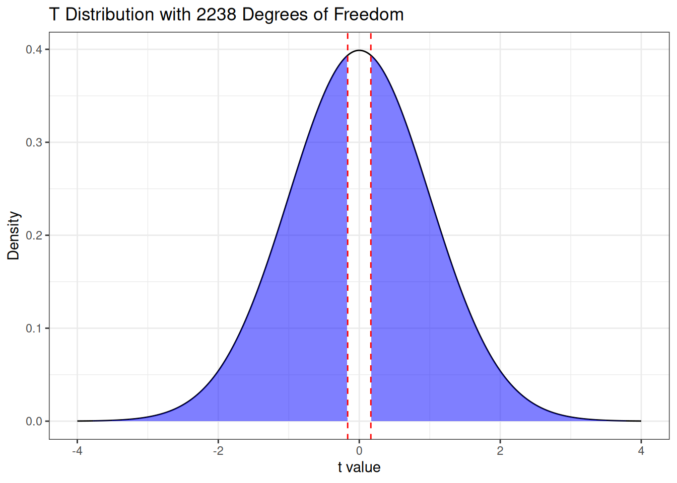
We can then compute the \(P\)-value as below:
t_stat_1 <- (1.0138985 - 1) / 0.08448966 ## These values are extracted from summary
2 * pt(q = t_stat_1, df = N - 2, lower.tail = FALSE)
[1] 0.8693529Because the \(P\)-value is close to 1, we can conclude that there is no evidence in the data that the true slope is not equal to 1.
6.6 Intervals for the Predicted Values
Rather than drawing inferences about the slope or intercept, we might want to make intervals that quantify our uncertainty directly about predictions that the model makes. For example, we might want to answer questions like the following one:
Question
On the GPA data, we estimate that a student with a high school GPA of 3.5 would have, on average, a first year GPA of 2.69. How precise is this prediction?
To answer this question, we need to clarify what exactly we mean by the prediction being “accurate.” We usually mean one of the following two things:
- For a single individual who happens to have a high school GPA of 3.5, what is a plausible range of first year GPAs they might have?
- Among the entire population of students who have a high school GPA of 3.5, what is a plausible range of values for the average first year GPA of these individuals?
Notice that the first is a statement about a single individual in the population (who happens to have a high school GPA of 3.5), whereas the second is a statement about a subpopulation of individuals (all of whom happen to have a high school GPA of 3.5, but may have different first year GPAs).
The interval associated with the first type of question is called a prediction interval, while the interval associated with the second type of question is called a confidence interval for the predicted value.
6.6.1 Confidence Intervals for the Predicted Values
Confidence intervals for predicted values quantify our uncertainty about the average outcome for a given value of the independent variable. For the GPA example, this would tell us about the plausible range for the average first-year GPA among all students with a particular high school GPA.
For a given value of the independent variable of interest \(x_0\), a confidence interval for the predicted value is:
\[ \widehat{Y}_0 \pm t_{\alpha/2} \times s_{\hat{Y}_0} \]
where \(\widehat{Y}_0 = \widehat\beta_0 + \widehat\beta_1 \, x_0\) is the predicted value and \(s_{\widehat{Y}_0}\) is the standard error of the predicted values, given by:
\[ s_{\widehat{Y}_0} = s \sqrt{\frac{1}{N} + \frac{(x_0 - \bar{X})^2}{SS_{XX}}} \]
Relationship with the Intercept
Notice that \(\beta_0\) also happens to be the predicted value when \(x_0 = 0\). As a sanity check, notice that when \(x_0 = 0\) the formula above gives \(s_{\widehat\beta_0}\).
Confidence intervals for predictions can be obtained using the predict() function by supplying the optional argument interval = "confidence". Let’s do this for our GPA example to get 95% confidence intervals:
## Get predictions and store them in an object fygpa_predictions
fygpa_predictions <- predict(fygpa_lm, interval = "confidence", level = 0.95)

## Print just the first few rows of fygpa_predictions
head(fygpa_predictions)
fit lwr upr
1 2.617990 2.576780 2.659199
2 3.063873 2.994866 3.132879
3 2.878088 2.822950 2.933227
4 2.878088 2.822950 2.933227
5 3.063873 2.994866 3.132879
6 3.063873 2.994866 3.132879This output gives us the predicted value (fit) and the lower and upper bounds of the 95% confidence interval. By default, this will give you confidence intervals for the data used to fit the regression. If you want to plug in new values you need to supply the newdata argument:
new_data <- data.frame(hs_gpa = 3.5)
predict(fygpa_lm, newdata = new_data, interval = "confidence", level = 0.95)
fit lwr upr
1 2.692304 2.648094 2.736513Interpretation: We are 95% confident that among all students with a high school GPA of 3.5, the average first-year college GPA is between 2.64 and 2.73.
6.6.2 Plotting Confidence Bands
In practice, it’s often useful to visualize these intervals across the range of the independent variable. We can do this in R as follows:
# Create a sequence of high school GPAs
hs_gpa_seq <- seq(0, 4.5, length = 200)

# Compute confidence intervals
ci_data <- predict(fygpa_lm, newdata = data.frame(hs_gpa = hs_gpa_seq),
                   interval = "confidence", level = 0.99999)

# Plot
plot(fygpa$hs_gpa, fygpa$fy_gpa,
     xlab = "High School GPA", ylab = "First Year College GPA",
     pch = 20, cex = 0.4)
lines(hs_gpa_seq, ci_data[,"fit"], col = "steelblue2", lwd = 2)
lines(hs_gpa_seq, ci_data[,"lwr"], col = "forestgreen", lty = 2, lwd = 2)
lines(hs_gpa_seq, ci_data[,"upr"], col = "forestgreen", lty = 2, lwd = 2)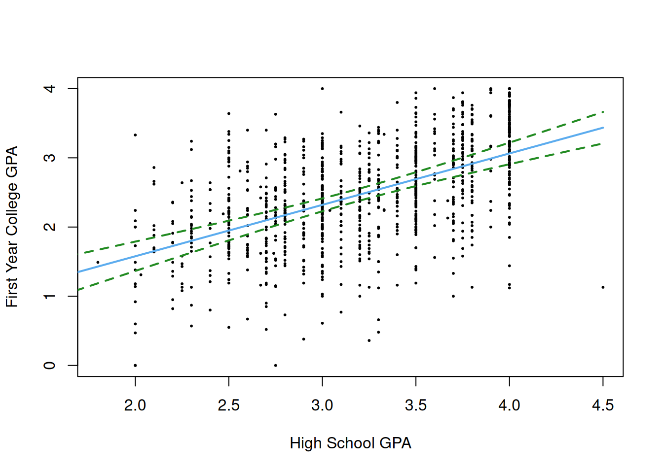
This displays both the fitted line (blue) and band around the fitted line (green) such that, for each high school GPA, we have a confidence interval for that specific value. Usually, I would make a 95% confidence band, but it turns out to be a little too narrow to see properly; to get a wider band, I instead made a 99.999% confidence band (a “five-nine” band2).
An interesting observation is that the confidence interval is narrower towards the center of the data and gets wider as we move away from the center; in fact, the band is narrowest when \(x_0 = \bar X\), which makes sense given the formula for \(s_{\widehat{Y}_0}\). This reflects the increased uncertainty in our predictions for values of \(X\) that are farther from the center of our data.
6.6.3 Prediction Bands
We now shift attention to the problem of predicting outcomes for an individual student rather than for an entire population of students. To see the difference between these two tasks, note that the 99.999% confidence bands for the regression line given above do not capture 99.999% of the students! To adequately put bounds on the score of an individual student, we need to consider two different sources of uncertainty:
- Uncertainty in the line (or equivalently, uncertainty in the values of \(\beta_0\) and \(\beta_1\)).
- Uncertainty in the behavior of an individual student, which would exist even if we knew the slope and intercept perfectly! Without this uncertainty, all of the students would appear exactly on the regression line.
More formally, let’s assume that there is a new student, who was not included in the sample, and we want to predict the student’s first year GPA \(Y_0\) given their high school GPA \(x_0\). We now want to choose the upper and lower endpoints of the interval so that
\[ \Pr(Y_0 \text{ is in the interval } ) = 1 - \alpha, \]
for some desired confidence level \(\alpha\). Such an interval is referred to as a prediction interval rather than a confidence interval. It turns out that the interval that does this is
\[ Y_0 = \widehat Y_0 \pm t_{\alpha/2} \times \sqrt{s^2 + s_{\widehat Y_0}^2} \]
where \(s_{\widehat Y_0}\) is the standard error for the predicted value \(\widehat Y_0\) that we used in constructing the confidence interval for the predicted value. This expression combines the two sources of uncertainty we noted above:
- \(s_{\widehat Y_0}^2\) accounts for uncertainty in estimating the regression line.
- \(s^2\) accounts for uncertainty in \(Y_0\), even if the regression line were known perfectly.
We can get prediction intervals in the exact same way we got confidence intervals; the only change required is that we need to change the argument interval = "confidence" to interval = "prediction". So, for example, we have
## This gets prediction intervals at each of the specified high school GPAs
predict(fygpa_lm, newdata = new_data, interval = "prediction", level = 0.95)
We can also get prediction intervals on new data using the newdata argument
new_data <- data.frame(hs_gpa = 3.5)
predict(fygpa_lm, newdata = new_data, interval = "prediction", level = 0.95)
fit lwr upr
1 2.692304 1.470493 3.914114Interpretation: We are 95% confident that a new student, who happens to have a high school GPA of 3.5, will have a first year GPA of between 1.47 and 3.91.
We can similarly make a prediction band that gives a prediction interval for each of the high school GPAs in the sample as follows:
# Create a sequence of high school GPAs
hs_gpa_seq <- seq(0, 4.5, length = 200)

# Compute prediction intervals
pi_data <- predict(fygpa_lm, newdata = data.frame(hs_gpa = hs_gpa_seq),
                   interval = "prediction", level = 0.95)

# Plot
plot(fygpa$hs_gpa, fygpa$fy_gpa,
     xlab = "High School GPA", ylab = "First Year College GPA",
     pch = 20, cex = 0.4)
lines(hs_gpa_seq, pi_data[,"fit"], col = "steelblue2", lwd = 2)
lines(hs_gpa_seq, pi_data[,"lwr"], col = "forestgreen", lty = 2, lwd = 2)
lines(hs_gpa_seq, pi_data[,"upr"], col = "forestgreen", lty = 2, lwd = 2)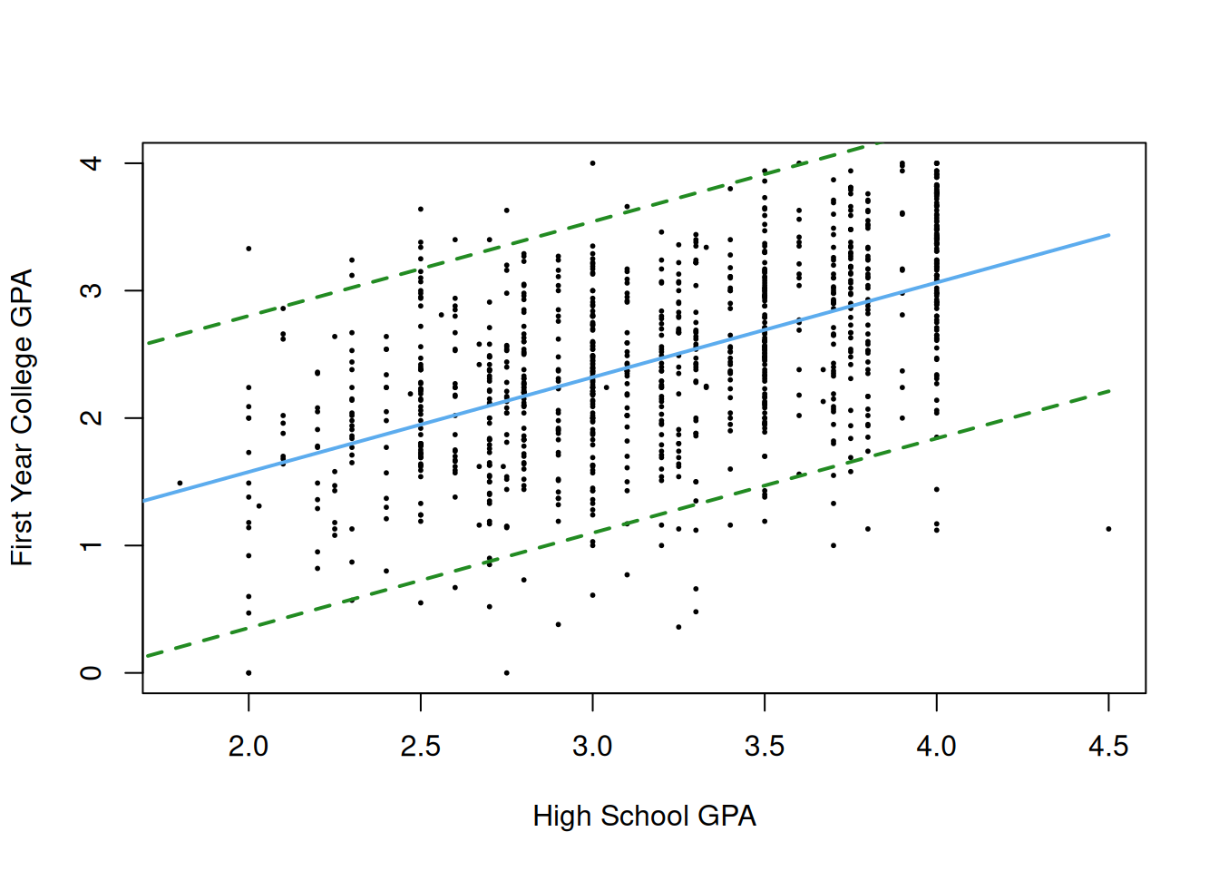
In this example, I reduced the prediction interval level from 99.999% to 95% because the 99.999% interval is too wide. We see that the 95% prediction interval is much wider than the confidence interval. This is because the interval has a different job than the confidence interval: it needs to catch a new student with probability 95%, and we can see from the above figure that the interval now does contain most of the data that we observed.
6.6.4 Intervals Using the broom package
Recall that the broom package also provides a function called augment() that does something very similar to the predict() function: it creates, for our original dataset, a data frame consisting of the observed independent variables, observed dependent variables, the predicted fitted values, and the residuals:
augment(fygpa_lm)# A tibble: 1,000 × 8
fy_gpa hs_gpa .fitted .resid .hat .sigma .cooksd .std.resid
<dbl> <dbl> <dbl> <dbl> <dbl> <dbl> <dbl> <dbl>
1 3.18 3.4 2.62 0.562 0.00114 0.622 0.000466 0.904
2 3.33 4 3.06 0.266 0.00319 0.622 0.000294 0.428
3 3.25 3.75 2.88 0.372 0.00204 0.622 0.000366 0.598
4 2.42 3.75 2.88 -0.458 0.00204 0.622 0.000555 -0.737
5 2.63 4 3.06 -0.434 0.00319 0.622 0.000781 -0.698
6 2.91 4 3.06 -0.154 0.00319 0.623 0.0000983 -0.248
7 2.83 2.8 2.17 0.658 0.00154 0.622 0.000864 1.06
8 2.51 3.8 2.92 -0.405 0.00224 0.622 0.000476 -0.652
9 3.82 4 3.06 0.756 0.00319 0.622 0.00237 1.22
10 2.54 2.6 2.02 0.517 0.00222 0.622 0.000769 0.831
# ℹ 990 more rowsIf we want, we can also tell the augment() function to also give confidence and/or prediction intervals by providing the optional argument interval = "confidence" or interval = "prediction". To get confidence intervals, for example, we have:
augment(fygpa_lm, interval = "confidence")# A tibble: 1,000 × 10
fy_gpa hs_gpa .fitted .lower .upper .resid .hat .sigma .cooksd .std.resid
<dbl> <dbl> <dbl> <dbl> <dbl> <dbl> <dbl> <dbl> <dbl> <dbl>
1 3.18 3.4 2.62 2.58 2.66 0.562 0.00114 0.622 4.66e-4 0.904
2 3.33 4 3.06 2.99 3.13 0.266 0.00319 0.622 2.94e-4 0.428
3 3.25 3.75 2.88 2.82 2.93 0.372 0.00204 0.622 3.66e-4 0.598
4 2.42 3.75 2.88 2.82 2.93 -0.458 0.00204 0.622 5.55e-4 -0.737
5 2.63 4 3.06 2.99 3.13 -0.434 0.00319 0.622 7.81e-4 -0.698
6 2.91 4 3.06 2.99 3.13 -0.154 0.00319 0.623 9.83e-5 -0.248
7 2.83 2.8 2.17 2.12 2.22 0.658 0.00154 0.622 8.64e-4 1.06
8 2.51 3.8 2.92 2.86 2.97 -0.405 0.00224 0.622 4.76e-4 -0.652
9 3.82 4 3.06 2.99 3.13 0.756 0.00319 0.622 2.37e-3 1.22
10 2.54 2.6 2.02 1.97 2.08 0.517 0.00222 0.622 7.69e-4 0.831
# ℹ 990 more rowsThe columns .lower and .upper now give the upper and lower bounds for the interval. Reading the results off from this, we can say:
- We are 95% confident that the population of students with high school GPA of 3.40 has an average first year GPA of between 2.58 and 2.66.
- We are 95% confident that the population of students with high school GPA of 4.00 has an average first year GPA of between 2.99 and 3.13.
- We are 95% confident that the population of students with high school GPA of 3.75 has an average first year GPA of between 2.82 and 2.93.
6.6.5 Assumptions Required for Prediction Bands
The validity of the prediction bands we have used requires that all of the Working Assumptions listed in this chapter hold. This makes them more fragile than the other intervals/bands/tests we have looked at, because we require that the errors \(\epsilon_i\) have a normal distribution (and this assumption cannot be made up for by having a large sample size).
6.6.5.1 Optional: Conformal Prediction
What should we do, then, if the normality assumption is wrong? Unfortunately there is no straight-forward answer here. There are other methods for making prediction intervals that make use of a technique called conformal prediction that is capable of producing prediction intervals that are valid even when all of the assumptions listed in this chapter are wrong. Of course, nothing in life is free, and describing conformal methods and their limitations is very far beyond the scope of this course.
6.7 What Are We Estimating if the Assumptions are Wrong
To recap, for Working Assumptions 2, 3, and 4, the consequences of being “wrong” about them are as follows.
Summary of Consequences of Violated Assumptions
If the errors are correlated, or if the errors are heteroscedastic, the standard errors of the \(\widehat\beta\)’s that you get from fitting a model using
lm()will be incorrect. This can be fixed using more advanced techniques, some of which we will learn in this class.If any of Assumptions 1, 2, or 3 are incorrect then Assumption 4 (normality of the residuals) is pointless, and it is more important to deal with the other assumptions first. But, if everything else looks OK, then Working Assumption 4 being wrong will not meaningfully affect statistical inferences about \(\beta_0\) and \(\beta_1\) provided that the sample size is large. It will, however, effect the accuracy prediction intervals regardless of the sample size, so if you want to make prediction intervals using the methods we will learn then you need the normality assumption to be correct.
Working Assumption 1 being wrong is a bit different than the others: without this assumption being correct, it is not even clear what we are estimating in the first place. What do the estimates \(\widehat \beta_0\) and \(\widehat \beta_1\) even mean if there isn’t actually any line to be estimated in the first place?
When the linearity assumption fails, the least squares estimators do still have a meaningful interpretation, albeit a different one from the usual linear regression context. In this case, \(\widehat \beta_0\) and \(\widehat \beta_1\) correspond to the best linear approximation to the true, non-linear, relationship. Revisiting the gas/temperature relationship, we can compare the linear and non-linear fits to each other:
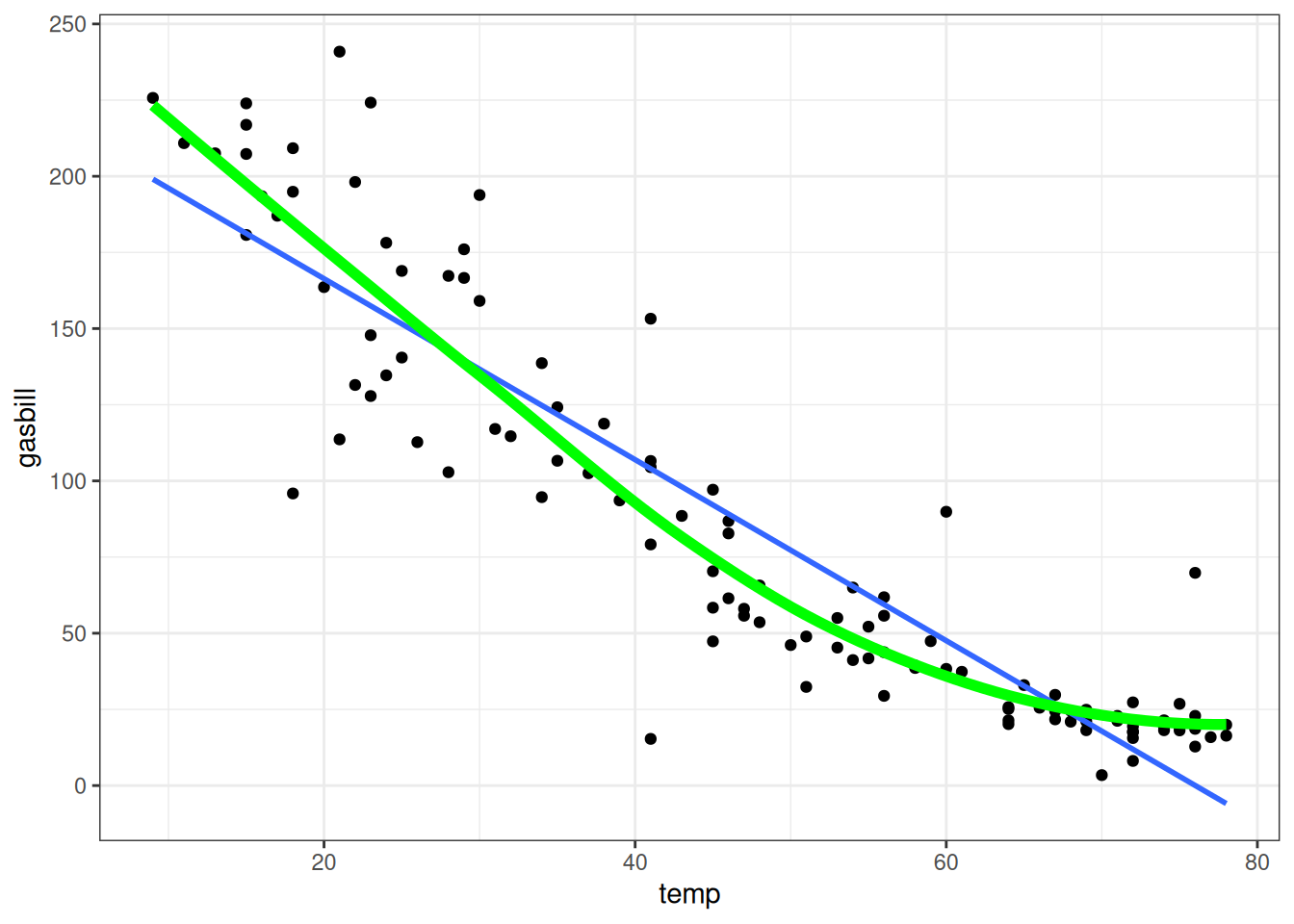
The important quantities at play here are:
- The relationship between \(Y_i = f(X_i) + \epsilon_i\) where \(f(x)\) is non-linear function and \(E(\epsilon_i) = 0\).
- Our non-linear estimate of \(f(x)\) is in green.
- There is also a best linear approximation \(\ell(x) = \beta_0 + \beta_1 \, x\) to \(f(x)\). It is the line that minimizes the approximation error \(E[\{\ell(X_i) - f(X_i)\}^2]\).
- The least-squares estimates \(\widehat\beta_0\) and \(\widehat \beta_1\) are now estimating the slope \(\beta_1\) and intercept \(\beta_0\) of the best-fitting line \(\ell(x)\).
So, while least squares is not estimating the actual relationship between \(X_i\) and \(Y_i\), it is at least estimating the best approximation to that relationship. Of course, it could be that \(\ell(x)\) is a bad approximation to \(f(x)\), in which case least squares will not be useful. But very frequently, even if the relationship is non-linear, it will be linear enough that we can still learn something about it from linear regression. For example, in the above figure, while the blue line does miss the curvature of the relationship it does seem to capture most of the relationship between temperature and gas bill. Depending on what our (scientific) goals are, a good line with a low approximation error might be good enough; in other contexts, where there are substantial non-linearity, it could be that the least squares is useless.
6.8 Exercises
6.8.1 Exercise: Boston Housing Data
The Boston housing dataset contains information on housing prices in various census tracts in Boston from the 1970s. The data can be loaded by running the following commands:
Boston <- MASS::BostonFit a simple linear regression model with
medv(median home value) as the dependent variable andnox(nitric oxide concentration) as the independent variable. Then, formulate an appropriate null hypothesis and alternative to test whethernoxis associated withmedv.Perform a test of the null hypothesis (against the alternative you specified). What \(P\)-value do you find? Does this \(P\)-value constitute strong evidence for or against the null?
Construct a 95% confidence interval for the slope \(\beta_{\text{nox}}\) in your regression model. Interpret the results.
Use the
augment()function to construct confidence intervals for the predicted values for the first 3 rows in the dataset. Then, give a careful interpretation of these confidence intervals, stating clearly what they correspond toRepeat part (d), but build prediction intervals instead.
6.8.2 Exercise: Advertising Data
We revisit the advertising dataset described below:
The advertising data set consists of sales of that product in 200 different markets. It also includes advertising budgets for the product in each of those markets for three different media: TV, radio, and newspapers.
Use the advertising dataset to answer the following questions:
advertising <- read.csv("https://www.statlearning.com/s/Advertising.csv")
advertising <- subset(advertising, select = -X)
Fit a simple linear regression model with
salesas the dependent variable andTVadvertising as the independent variable. Then, test whether TV advertising is predictive of sales; state clearly the model you are fitting and the null/alternative hypotheses. Based on the \(P\)-value, how strong is your evidence against the null hypothesis?Plot
TVon the x-axis andsaleson the y-axis. Which (if any) of the working assumptions appear to be violated?For the assumptions you identified in the previous part that were violated, state what the consequences are of the violation of these assumptions on the conclusions you can draw.
Construct a 95% confidence interval for the slope \(\beta_1\) of the TV advertising data. Interpret the interval in context. What does this say about the effect of each additional thousand dollars spent on TV advertising?
Plot a figure displaying:
- a scatterplot displaying
sales(dependent variable) againstTV(independent variable); - the line giving the estimated linear relationship between
TVandsales; - a 95% confidence band for the predicted values;
- a 95% prediction band for new observations.
Then, explain clearly the difference between the confidence band and the prediction band; why is the prediction band wider?
- a scatterplot displaying
Also construct a 95% confidence interval for the slope \(\beta_1\) with
radioadvertising as the predictor andsalesas the outcome. Compare the interval with the one obtained for TV advertising. Which medium appears to have a more predictable effect on sales?
6.8.3 Exercise: Affairs Data
Using the Affairs dataset from the AER package in R, we’ll explore the relationship between marriage rating and the frequency of extramarital affairs. The data can be loaded by running the following commands:
# Load the data
library(AER)
data("Affairs")

head(Affairs)
affairs gender age yearsmarried children religiousness education occupation
4 0 male 37 10.00 no 3 18 7
5 0 female 27 4.00 no 4 14 6
11 0 female 32 15.00 yes 1 12 1
16 0 male 57 15.00 yes 5 18 6
23 0 male 22 0.75 no 2 17 6
29 0 female 32 1.50 no 2 17 5
rating
4 4
5 4
11 4
16 5
23 3
29 5Details on the individual columns of this dataset can be obtained by running ?Affairs. Use simple linear regression to answer the following questions.
- Fit a simple linear regression model where the dependent variable is the number of affairs and the independent variable is the marriage rating. Test whether the marriage rating is a significant predictor of the number of affairs. State your hypotheses and interpret the result.
- Construct a 95% confidence interval for the slope \(\beta_1\) in this model. Interpret the results.
- For marriage ratings of 3 and 4, construct a 95% confidence interval for the average affair frequency. Interpret the interval.
- For marriage ratings of 3 and 4, construct a 95% prediction interval for the number of affairs for a new individual. Explain the difference between this interval and the one in part (c).
6.8.4 Exercise: Assumption Violations
Given the scenarios described below, identify which working assumption(s) for linear regression might be violated. Provide a brief explanation for your identification.
Scenario 1: You are analyzing data in which the amount of rainfall (in inches) on a given day is being used to predict the next day’s temperature (in degrees Fahrenheit). However, you notice that on extremely rainy days, the temperature the next day is more variable than on dry days.
Scenario 2: In a study aiming to predict students’ performance based on hours studied, you find that students who attended the same study group show similar deviations from the predicted performance, regardless of the hours they studied.
Scenario 3: Researchers are analyzing the relationship between exercise duration (hours per week) and weight loss (pounds). However, they find that for individuals exercising more than 10 hours a week, the additional weight loss effect is diminishing and appears curved rather than linear.
6.8.5 Exercise: Statistical Inference By Hand
In this exercise, you’ll manually perform the tasks of constructing a confidence interval and conducting a hypothesis test for the slope and intercept of a linear regression model. Assume you have the following information from a regression analysis of a dataset with \(N = 100\) observations:
- \(\bar{X} = 5.8\)
- \(\bar{Y} = 3.06\)
- \(SS_{XX} = 102.2\)
- \(SS_{XY} = 28.3\)
- The sum of squared residuals \(\sum e_i^2\) is 27.9.
Estimate the Regression Coefficients:
- Calculate the slope (\(\widehat{\beta}_1\)).
- Calculate the intercept (\(\widehat\beta_0\)).
Compute the Standard Errors:
- Calculate the residual standard error (\(s\)).
- Calculate the standard error of \(\widehat\beta_0\) (\(s_{\widehat\beta_0}\)).
- Calculate the standard error of \(\widehat\beta_1\) (\(s_{\widehat\beta_1}\)).
Construct a 95% Confidence Interval for \(\beta_1\):
Conduct a Hypothesis Test for \(\beta_1\):
- Test the null hypothesis (\(H_0: \beta_1 = 0\)) against the alternative (\(H_1: \beta_1 \ne 0\)).
- Calculate the \(T\)-statistic.
- Determine the \(P\)-value and state how strong the evidence is against the null hypothesis.
Construct a 95% Confidence Interval for \(\beta_0\):
Conduct a Hypothesis Test for \(\beta_0\):
- Perform the same hypothesis test as for \(\beta_1\), and state your conclusions.
Available for free here: http://www.stat.columbia.edu/~gelman/book/BDA3.pdf↩︎
I borrowed this term from https://www.argmin.net/p/randomly-revealing-hidden-truths, who attributes it to folks from reliability engineering and computer science.↩︎