A limitation of multiple linear regression is that it requires that the dependent variable is numeric. While this setting is very common, in many fields it is equally common to have a dependent variable be qualitative. Examples include:
Whether a patient survives a medical procedure (survived/died).
The marital status of an individual (married/divorced/widowed).
Whether a student is admitted to a university (admitted/rejected).
The party chosen by a voter (Democrat/Republican/Independent).
These are all examples where the quantity we want to predict is qualitative, and in each case we would most likely be interested in modeling the probability of one of the possible categories versus the others.
To properly deal with qualitative dependent variables, we need different tools. In this chapter, we will deal with the special case of outcomes that take on two possible values, one of which is referred to as a “success” and the other referred to as a “failure.” This includes the first and third examples given above. To do this, we will introduce the logistic regression model.
15.1 Why Do We Need Logistic Regression?
As an alternative to using a new method, we might hope to handle this type of data by using linear regression. We were able to do this when handling qualitative independent variables by using dummy variables, which let us treat qualitative variables as numeric; maybe a similar trick will work for dependent variables. Specifically, suppose that \(Y_i\) takes two levels and we set \(Y_i = 1\) for a success and \(Y_i = 0\) for a failure. Then we could apply a linear regression model
using the same workflow with lm() as before. This turns out not to work very well. The reason we need different tools is because the assumptions underlying statistical inference for linear regression are inherently violated for qualitative data:
The relationship between \(Y_i\) and the \(X_{ij}\)’s is usually not linear; one way to see this is that if we took the model above and plugged in large \(X_{ij}\)’s then we might get predictions for \(Y_i\) that either exceed 1 or are negative. So the linearity assumption is (usually) violated.
It turns out that for data with only two levels, the variance of the error is related to the predicted value of \(Y_i\). Specifically, if \(Y_i\) has average \(p_i\), then it is a mathematical fact that the variance of \(Y_i\) is \(p_i (1 -
p_i)\). So the constant variance assumption is violated.
It goes without saying that if \(Y_i\) can only take the values \(0\) or \(1\) then it cannot possibly have a normal distribution. So the normality assumption on the errors is violated.
Because of this, if we apply linear regression then we probably cannot have a lot of faith in the results we get, at least as far as statistical inference is concerned. Instead of trying to correct these issues, it is more expedient to just use a model that is specifically designed for qualitative outcomes.
15.2 Motivating Example: The Challenger Shuttle
On January \(28^{\text{th}}\), 1986, the space shuttle Challenger broke apart just after launch, taking the lives of all seven crew members. This example is taken from an article by Dalal et al. (1989), which tried to determine whether the incident could have been predicted, and hence prevented, on the basis of data from previous flights. The cause of failure was ultimately attributed to the failure of a crucial shuttle component known as the O-rings; these components had been tested prior to the launch to see if they could hold up under a variety of temperatures.
The dataset Challenger.csv consists of data from test shuttle flights. This can be loaded using the following commands.
The variables of importance for this analysis are Temperature (the ambient temperature on the day of an O-ring test) and Fail (whether at least one O-ring failed during the test).
Our Goal: The substantive question we are interested in is whether those in charge of the Challenger launch should have known that the launch was dangerous and delayed it until more favorable weather conditions. In fact, engineers working on the shuttle had warned beforehand that the O-rings were more likely to fail at lower temperatures. To determine this, we will try to estimate how the probability of O-ring failure varies with the temperature.
15.3 The Binomial Distribution
Rather than following a normal distribution, when the outcomes can only take one of two values it is more appropriate to use a binomial distribution. We now discuss this, which can be used to represent the results of experiments consisting of successes and failures. A binomial random variable \(Y_i\) is characterized by two quantities:
\(p_i\): the probability of a success (with \(1 - p_i\) being the probability of a failure).
\(n_i\): the number of trials in the experiment.
Example: Flipping a Coin
Suppose I flip a fair coin \(10\) times and record \(Y_i\) as the number of heads, regarding a coin landing “heads” as a success and landing “tails” as a failure. Then \(Y_i\) will have a binomial distribution with \(p_i = 0.5\) and \(n_i = 10\). If, instead, the coin was unfair (landing, say, heads 60% of the time) and I flipped it 30 times then \(Y_i\) would be binomial with \(p_i = 0.6\) and \(n_i =
30\).
Given these parameters, the probability that \(Y_i\) takes any particular value \(y\) between \(0\) and \(n_i\) is given by
where \(\binom{n_i}{y} = \frac{n_i!}{y! (n_i - y)!}\) is referred to as a binomial coefficient, which represents the number of different ways of getting \(y\) successes across the \(n_i\) independent trials.
Example: Flipping a Fair Coin
To give some intuition on the formula above, let’s directly compute the probabilities associated to the number of heads we see if a coin lands heads assuming \(n_i = 3\) trials are done and the coin lands heads with probability \(p_i\).
There is only one way to flip no heads (TTT), and this occurs with probability \((1 - p_i)^3\).
There are three ways to flip exactly on heads (TTH, THT, HTT), and each occurs with probability \(p_i (1 - p_i)^2\).
There are three ways to flip exactly two heads (THH, HTH, HHT), and each occurs with probability \(p_i^2 (1 - p_i)\).
There is only one way to flip three heads (HHH), and this occurs with probability \(p_i^3\).
Checking this against the general formula we gave, the formula matches because \(\binom{3}{0} = 1\), \(\binom{3}{1} = 3\), \(\binom{3}{2} = 3\), and \(\binom{3}{3} = 1\).
In the case of the Challenger dataset, each O-ring test can be viewed as a binomial experiment with \(n_i = 1\), where success (\(Y_i = 1\)) represents a malfunction of the O-ring and a failure (\(Y_i = 0\)) represents no O-ring malfunction. This special case of the binomial distribution where \(n_i = 1\) is often called a Bernoulli distribution. The probability of failure \(p_i\) is what we want to model as a function of temperature. Our goal will be to model how this probability \(p_i\) changes with temperature, which will allow us to assess whether launching the Challenger at low temperatures substantially increased the risk of O-ring failure.
15.4 The Logistic Regression Model
The go-to model for binomial outcomes is called logistic regression. In this model, the probability of success \(p_i\) is related to the independent variables through the equation
(Reminder: \(e \approx 2.71\) is the base of the natural logarithm).
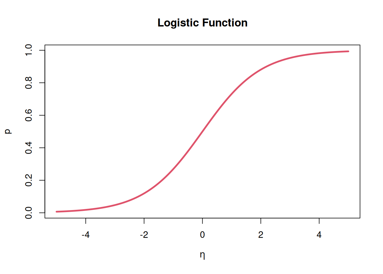
The quantity \(\eta_i\), called the linear predictor, combines the effects of all independent variables in a linear fashion. However, rather than directly relating this linear combination to the probability of success, we transform it using what is known as the logistic function\(e^\eta / (1 + e^\eta)\), shown in the plot below:
The logistic function has several important properties that make it suitable for modeling probabilities. First, it transforms any number \(\eta_i\) into a value between 0 and 1, which is necessary since probabilities must lie in this range. This addresses the issue with linear regression we saw, where we want to avoid predicting probabilities bigger than 1 or less than 0. Second, it has an “S-shaped” form: when \(\eta_i\) is very negative the probability approaches 0, when \(\eta_i\) is very positive the probability approaches 1, and there is a smooth transition between these extremes. This behavior naturally models many real-world phenomena where the effect of changing the independent variables is most pronounced near \(p_i = 0.5\) and diminishes as we approach either extreme.
As with linear regression, some assumptions are required for inferences from the logistic regression model to be valid:
Linearity: The quantity \(\eta_i\) should depend linearly, i.e., \(\eta_i = \beta_0 + \sum_{j=1}^P \beta_j \, X_{ij}\).
Independence Across Observations: The \(Y_i\)’s should be independent of each other, i.e., what happens to one of the outcomes should not influence the other outcomes. In the context of the Challenger data, this means that the outcome of one O-ring test does not influence the outcomes of other tests.
Independent Trials: If \(n_i > 1\) (so that \(Y_i\) is associated with more than one success/failure), each of the successes/failures associated with \(Y_i\) should be independent of each other. For example, if I am flipping a coin \(n_i = 3\) times, then whether I get heads on the first flip should not affect the probability of getting heads on the second flip.
We will assume throughout this chapter that all of these assumptions are satisfied.
15.5 The Principle of Maximum Likelihood
While linear regression models are fit using the principle of least squares, logistic regression models are typically fit using a different approach called maximum likelihood. The key idea behind maximum likelihood is to choose the coefficients that make our observed data as probable as possible under the model.
To make this concrete, suppose we have estimated coefficients \(\widehat\beta_0, \widehat\beta_1, \ldots, \widehat\beta_P\) which give us estimated probabilities
These estimated probabilities allow us to compute the estimated probability of observing each outcome in our dataset. Because we assume the observations are independent, we can multiply these probabilities together to get the probability of observing our entire dataset:
This quantity \(L\) is called the likelihood of the data. Maximum likelihood estimation simply chooses the coefficients \(\widehat\beta_j\) that make this likelihood as large as possible.
For the Challenger data, since we have binary outcomes (\(n_i = 1\)), this simplifies to
where \(Y_i = 1\) indicates an O-ring failure and \(Y_i = 0\) indicates no failure. The coefficients we choose will determine the probabilities \(p_i\) through the logistic regression equation.
15.5.1 Illustration: Simple Logistic Regression
To illustrate the concept, let’s look at performing maximum likelihood on the Challenger data. The following function defined in R computes the likelihood for a simple logistic regression model (i.e., the model with \(P = 1\)):
likelihood_challenger <-function(beta) {# Extract coefficients beta0 <- beta[1] beta1 <- beta[2]# Compute linear predictor eta <- beta0 + beta1 * challenger$Temperature# Transform to probabilities p <-exp(eta) / (1+exp(eta))# Compute log-likelihood log_lik <-sum(challenger$Fail *log(p) + (1- challenger$Fail) *log(1- p))## The likelihood is the exponential of the log-likelihoodreturn(exp(log_lik))}
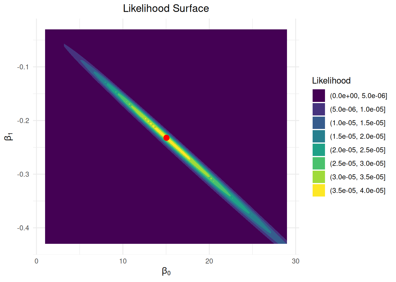
Because there are only two things we need to estimate (\(\beta_0\) and \(\beta_1\)), we can visualize this function using a contour plot:
# Create grid of beta valuesgs <-90beta0_grid <-seq(15-2*7, 15+2*7, length = gs)beta1_grid <-seq(-0.23-2*0.1, -0.23+2*0.1, length = gs)grid <-expand.grid(beta0 = beta0_grid, beta1 = beta1_grid)# Compute likelihood for each pairgrid$likelihood <-sapply(1:nrow(grid), \(i) likelihood_challenger(c(grid$beta0[i], grid$beta1[i])))# Get MLE for plottingfit <-glm(Fail ~ Temperature, data = challenger, family = binomial)mle <-coef(fit)# Create filled contour plotggplot(grid, aes(x = beta0, y = beta1, z = likelihood)) +geom_contour_filled() +geom_point(data =data.frame(beta0 = mle[1], beta1 = mle[2], likelihood =0),aes(x = beta0, y = beta1),color ="red", size =3) +scale_fill_viridis_d(name ="Likelihood") +labs(x =expression(beta[0]), y =expression(beta[1]),title ="Likelihood Surface") +theme_minimal() +theme(plot.title =element_text(hjust =0.5))
To read the contour plot, the \(x\)-axis gives a particular possible value of \(\beta_0\), the \(y\)-axis gives a possible value of \(\beta_1\), and the color tells us how big the likelihood is at that combination; the maximum likelihood estimator is then given by the “most yellow” point on the contour (which has been highlighted in red).
We see that the maximum is obtained around \(\widehat \beta_0 = 15.0429\) and \(\widehat \beta_1 = -0.2322\). These are the values that make the data that we observed as likely to observe as possible. Values of \(\beta_0\) and \(\beta_1\) outside the range of this plot correspond to values that make the data we observed increasingly implausible.
15.5.2 Some Details on Implementing Maximum Likelihood
In practice, unlike with linear regression, there is no exact formula to get the \(\widehat \beta_j\)’s. While we were able to visualize the likelihood surface for a simple logistic regression with one predictor, this becomes impossible when we have multiple predictors since we cannot visualize surfaces in more than three dimensions. Moreover, even in the simple case, finding the exact maximum by visual inspection would be imprecise.
Instead, we must rely on numerical optimization methods to find the maximum likelihood estimates. The approach used in R employs Newton’s method to find the optimum. (Optional: see here for a description of Newton’s method). The mathematical details of why this works involve calculus and numerical optimization theory, but the key insight is that we can systematically improve our parameter estimates by looking at the local behavior of the likelihood surface, even when we can’t visualize it directly.
15.6 Interpreting the Coefficients of the Logistic Regression Model
Unlike linear regression where the coefficients represent direct changes in the response variable, interpreting logistic regression coefficients is less straightforward due to the nonlinear relationship between predictors and probabilities. Fortunately, we can get a relatively simple interpretation of the \(\beta_j\)’s regardless.
The most natural interpretation of logistic regression coefficients comes through a quantity called the odds of success, defined as:
\[
o_i = \frac{p_i}{1 - p_i}
\]
While less intuitive than probabilities, odds are often used in gambling contexts:
Odds of 3-to-1 means \(o_i = 3\), corresponding to probability \(p_i = 0.75\) (since \(0.75/0.25 = 3/1\))
Odds of 3-to-2 means \(o_i = 1.5\), corresponding to probability \(p_i = 0.60\) (since \(0.60/0.40 = 3/2\))
Odds of 1-to-4 means \(o_i = 0.25\), corresponding to probability \(p_i = 0.20\) (since \(0.20/0.80 = 1/4\))
To see why odds are natural for logistic regression, note that if we solve the logistic regression equation for the odds, we get:
Holding all other independent variables constant, increasing \(X_{ij}\) by one unit leads to multiplying the odds of success by \(e^{\beta_j}\).
For example, if \(\beta_j = 2\) then increasing \(X_{ij}\) by one units results in multiplying the odds of success by \(e^2 = 7.389\).
15.6.1 Example: The Challenger Data
Let’s interpret \(\beta_1\) for the Challenger dataset. Earlier we obtained the estimate \(\widehat \beta_1 = -0.2322\) by maximizing the likelihood function. This leads to the following interpretation:
Given a one degree increase in temperature, the estimated odds of an O-ring failure is multiplied by \(e^{-0.2322} \approx 0.8\).
We can also talk about shifts of more than one unit. For example:
Given a ten degree decrease in temperature, the estimated odds of an O-ring failure is multiplied by \(e^{-10 \times -0.2322} \approx 10.2\).
So, roughly speaking, each ten degree decrease in temperature increases the estimated odds of an O-ring failure by a factor of 10.
15.7 The glm Function
In R, logistic regression is implemented as part of a broader class of models called Generalized Linear Models (GLMs). The function glm() provides a unified interface for fitting these models, with the family argument specifying which type of model we want to fit. Let’s look at how to handle each case.
15.7.1 Binary Outcomes
Fitting a logistic regression in R is similar to fitting a linear regression: we plug a formula and a dataset into the function glm. Let’s fit a model to the Challenger data:
# Fit logistic regressionchallenger_glm <-glm(Fail ~ Temperature, data = challenger, family = binomial)
There is one additional argument that we need to provide: the family = binomial argument specifies that we want to fit a logistic regression model. The glm() function (which stands for Generalized Linear Model) is actually capable of fitting several other types of models, including:
family = gaussian: Standard linear regression
family = binomial: Logistic regression
family = poisson: Poisson regression (which we’ll see in the next chapter)
After fitting the model we can use the summary() function to get the results:
# View the summarysummary(challenger_glm)
Call:
glm(formula = Fail ~ Temperature, family = binomial, data = challenger)

Coefficients:
            Estimate Std. Error z value Pr(>|z|)
(Intercept)  15.0429     7.3786   2.039   0.0415 *
Temperature  -0.2322     0.1082  -2.145   0.0320 *
---
Signif. codes:  0 '***' 0.001 '**' 0.01 '*' 0.05 '.' 0.1 ' ' 1

(Dispersion parameter for binomial family taken to be 1)

    Null deviance: 28.267  on 22  degrees of freedom
Residual deviance: 20.315  on 21  degrees of freedom
AIC: 24.315

Number of Fisher Scoring iterations: 5
The summary output provides several important pieces of information:
The estimated coefficients (\(\widehat\beta_j\)’s) and their standard errors
\(Z\)-statistics and \(P\)-values for testing whether each coefficient is zero; these are directly analogous to the tests performed when looking at the output of summary() for a model fit with lm().
The null and residual deviance, which measure model fit; we will discuss these later.
The AIC (Akaike Information Criterion) for model comparison.
The number of iterations of Newton’s method that were used to fit the model (5 in this case).
15.7.2 Binomial Outcomes
In some cases, rather than having a binary outcome (as with the Challenger dataset), we might have a binomial outcome where we observe the number of successes out of a fixed number of trials. For example, the Challenger dataset actually contains information on the number of O-ring failures that occurred, out of a possible 6 O-rings. The number of failures is given by the nFailures column.
To handle binomial outcomes in glm() with \(n_i > 1\) we need to instead specify response as follows:
# Create response matrix for O-ring failuresY_failures <-cbind(challenger$nFailures, 6- challenger$nFailures) # 6 minus failures = non-failures# Fit modelfailures_glm <-glm(Y_failures ~ Temperature, family = binomial,data = challenger)summary(failures_glm)
Call:
glm(formula = Y_failures ~ Temperature, family = binomial, data = challenger)

Coefficients:
            Estimate Std. Error z value Pr(>|z|)
(Intercept)  5.08498    3.05247   1.666   0.0957 .
Temperature -0.11560    0.04702  -2.458   0.0140 *
---
Signif. codes:  0 '***' 0.001 '**' 0.01 '*' 0.05 '.' 0.1 ' ' 1

(Dispersion parameter for binomial family taken to be 1)

    Null deviance: 24.230  on 22  degrees of freedom
Residual deviance: 18.086  on 21  degrees of freedom
AIC: 35.647

Number of Fisher Scoring iterations: 5
The interpretation of this model is the same as before - increasing Temperature by 1 degree leads to multiplying the odds of an O-ring failing by \(e^{-0.1156} \approx 0.9\) - but now we are modeling the probability of an individual O-ring (of six) failing rather than the probability of at least one failure.
15.8 Getting the Predictions from the Model
After fitting a logistic regression, we often want to obtain estimated probabilities for various values of our independent variables. The estimated probability of success for each observation is given by
In R, we can compute the estimated probabilities using the predict() function:
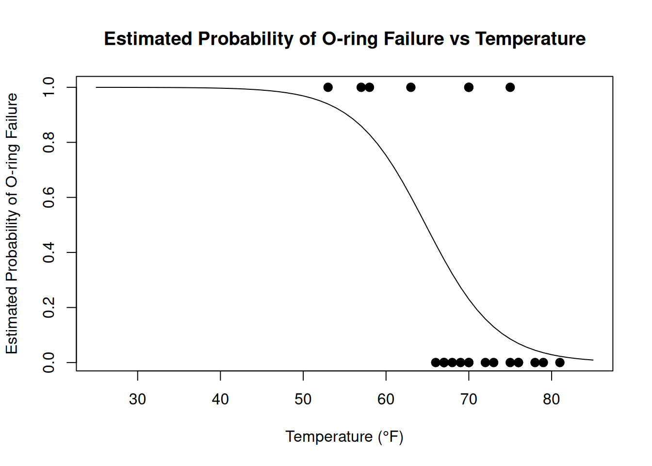
# Create sequence of temperatures for predictiontemps <-seq(from =25, to =85, by =1)# Get predicted probabilitiesprobs <-predict(challenger_glm, newdata =data.frame(Temperature = temps), type ="response")
Warning
It is important to include the argument type = "response" to the predict() function; failure to include this results in predict() returning the quantity \(\widehat \eta_i = \widehat \beta_0 + \sum_{j=1}^P \widehat\beta_j \, X_{ij}\).
After doing this, we can plot the estimated probabilities along with the successes and failures:
# Create visualizationplot(temps, probs,type ='l',xlab ="Temperature (°F)", ylab ="Estimated Probability of O-ring Failure",main ="Estimated Probability of O-ring Failure vs Temperature")# Add successes and failurespoints(challenger$Temperature, challenger$Fail,pch =19,cex =1.2)
This visualization shows that, generally, as the temperature decreases, the estimated probability that there will be an O-ring failure steadily increases to 1.
We can also use predict() to answer specific questions. For example, the estimated probability of failure at the temperature on the day of the Challenger launch was:
predict(challenger_glm, newdata =data.frame(Temperature =31), type ="response")
        1
0.9996088
or 99.96%. This concerning estimate aligns with the warnings that engineers gave before the launch about the dangers of launching at such low temperatures.
Extrapolation
In addition to the estimated probability of failure being extremely high, predicting at a temperature of 31 degrees requires a massive extrapolation! Because of this:
We should be skeptical of trusting the 99.96% number.
We should probably err on the side of being even more wary of doing a launch in such conditions, which are way beyond what the shuttle was ever tested.
15.9 Statistical Inference With Logistic Regression Models
For the most part, statistical inference for logistic regression is very similar to statistical inference for linear regression. Let’s again plot the output of summary() for reference:
summary(challenger_glm)
Call:
glm(formula = Fail ~ Temperature, family = binomial, data = challenger)

Coefficients:
            Estimate Std. Error z value Pr(>|z|)
(Intercept)  15.0429     7.3786   2.039   0.0415 *
Temperature  -0.2322     0.1082  -2.145   0.0320 *
---
Signif. codes:  0 '***' 0.001 '**' 0.01 '*' 0.05 '.' 0.1 ' ' 1

(Dispersion parameter for binomial family taken to be 1)

    Null deviance: 28.267  on 22  degrees of freedom
Residual deviance: 20.315  on 21  degrees of freedom
AIC: 24.315

Number of Fisher Scoring iterations: 5
15.9.1 Hypothesis Testing
To test for whether temperature is related to the probability of O-ring failure, we can formulate the following null and alternative hypotheses:
\(H_0\): \(\beta_1 = 0\)
\(H_1\): \(\beta_1 \ne 0\)
A \(P\)-value for this test appears in the output of summary(), and seems to be 0.0320. So there is some evidence that temperature is associated with the probability of an O-ring failure; the result is significant if we use a \(P\)-value cutoff of 0.05, but not if we use a more stringent cutoff of (say) \(0.01\).
It turns out, however, that the output of summary()does not produce an accurate\(P\)-value. A better \(P\)-value can be obtained using either anova() (to perform sequential tests) or drop1() (to perform single-term deletion tests). Using drop1() we get:
drop1(challenger_glm, test ="LRT")
Single term deletions

Model:
Fail ~ Temperature
            Df Deviance    AIC   LRT Pr(>Chi)
<none>           20.315 24.315
Temperature  1   28.267 30.267 7.952 0.004804 **
---
Signif. codes:  0 '***' 0.001 '**' 0.01 '*' 0.05 '.' 0.1 ' ' 1
When using this more appropriate test, we get a \(P\)-value of 0.0048, which gives us substantially stronger evidence against the null hypothesis.
The test Argument
The appropriate argument to test when fitting a logistic regression is test = "LRT". This tells drop1() to perform a likelihood ratio test, which is the appropriate test to use for logistic regression.
Don’t Use the P-Values in Summary
Unlike with linear regression, generally the \(P\)-values obtained with summary() are untrustworthy. There are situations where, for example, they incorrectly give a \(P\)-value close to 1 while anova() or drop1() correctly give a \(P\)-value close to 0.
15.9.2 Testing for Overall Model Significance
Just as with linear regression, we often want to test whether our model as a whole is providing a significant fit to the data. For logistic regression, this involves comparing our model to a “null model” that includes only an intercept term. That is, we are interested in testing the following hypotheses:
\(H_1\): At least one of the \(\beta_j\)’s is not equal to \(0\).
One way to do this is to use the anova() function to compare the model we have fit to a model that only uses the intercept \(\beta_0\). For the Challenger dataset, we can first fit the model that includes only an intercept:
## Fit the intercept-only challenger modelchallenger_intercept <-glm(Fail ~1, data = challenger, family = binomial)
Then we can use anova() to compare this to our original model:
## Use anova() to compare intercept-only to the model that uses Temperatureanova(challenger_intercept, challenger_glm, test ="LRT")
Analysis of Deviance Table

Model 1: Fail ~ 1
Model 2: Fail ~ Temperature
  Resid. Df Resid. Dev Df Deviance Pr(>Chi)
1        22     28.267
2        21     20.315  1    7.952 0.004804 **
---
Signif. codes:  0 '***' 0.001 '**' 0.01 '*' 0.05 '.' 0.1 ' ' 1
The results here are the same as what we got from drop1() because there is only one independent variable; the result would be different if we had more than one independent variable.
Relationship to drop1()
For models with a single predictor like our Challenger example, this overall significance test gives the same result as using drop1(). For models with multiple predictors, the overall significance test examines whether any of the predictors are useful, while drop1() tests the significance of each predictor individually.
15.9.3 Confidence Intervals
If we want a confidence interval for the coefficients, we can use the confint() function, just like we did with linear regression:
confint(challenger_glm, level =0.95)
                 2.5 %      97.5 %
(Intercept)  3.3305848 34.34215133
Temperature -0.5154718 -0.06082076
Based on this output we can conclude the following:
We are 95% confident that increasing the temperature by one unit leads to multiplying the odds of an O-ring failure occurring by between \(e^{-0.5154718} \approx 0.597\) and \(e^{-0.06082076} \approx 0.941\).
Or, in terms of a 10 degree decrease in temperature:
We are 95% confident that decreasing the temperature by ten units leads to multiplying the odds of an O-ring failure occuring by between \(e^{5.154718} \approx 173.2\) and \(e^{0.6082076} \approx 1.8\).
So, while there is substantial evidence that decreasing temperature tends to increase the odds of an O-ring failure, there is substantial uncertainty about how much decreasing the temperature increases these odds.
15.9.4 Confidence Bands
Finally, we will consider quantifying our uncertainty in our estimated relationship between temperature and the probability of an O-ring failure occurring. This turns out to be a bit more tricky to do than getting a confidence band for linear regression:
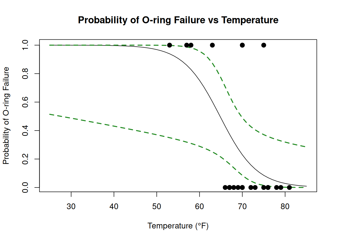
# Create sequence of temperatures for predictiontemps <-seq(from =25, to =85, by =1)# Get predicted probabilitiesprobs <-predict(challenger_glm, newdata =data.frame(Temperature = temps), type ="response")# Get confidence intervals on link scalepreds_link <-predict(challenger_glm,newdata =data.frame(Temperature = temps),type ="link",se.fit =TRUE)# Convert to response scaleci_lower <-plogis(preds_link$fit -1.96* preds_link$se.fit)ci_upper <-plogis(preds_link$fit +1.96* preds_link$se.fit)# Create visualizationplot(temps, probs, type ="l",xlab ="Temperature (°F)", ylab ="Probability of O-ring Failure",main ="Probability of O-ring Failure vs Temperature")lines(temps, ci_lower, col ='forestgreen', lty =2, lwd =2)lines(temps, ci_upper, col ='forestgreen', lty =2, lwd =2)# Add observed data pointspoints(challenger$Temperature, challenger$Fail,pch =19,cex =1.2)
The dashed lines above are a 95% confidence band, giving an interval around where the actual probability at each temperature should lie. Again, there is a lot of uncertainty!
Sadly, the predict() function doesn’t give these bands directly. Instead what we do is
Get estimates \(\widehat \eta = \widehat \beta_0 + \sum_{j = 1}^P \widehat\beta_j \, X_{ij}\) using type = "link" with standard errors (se.fit = TRUE)
Construct a 95% confidence interval for the linear predictor: \[
\eta_i = \widehat \eta_i \pm 1.96 \times s_{\widehat \eta_i}
\]
Transform these confidence limits back to the probability scale using the logistic function: \[
p_i = \frac{e^{\eta_i}}{1 + e^{\eta_i}}
\]
This process explains the code we used above:
# Get confidence intervals on link scalepreds_link <-predict(challenger_glm,newdata =data.frame(Temperature = temps),type ="link",se.fit =TRUE)# Convert to response scale using plogis() (the logistic function)ci_lower <-plogis(preds_link$fit -1.96* preds_link$se.fit)ci_upper <-plogis(preds_link$fit +1.96* preds_link$se.fit)
The reason we need to do this transformation is that confidence intervals constructed directly on the probability scale can sometimes give invalid probabilities (less than 0 or greater than 1). By constructing the intervals on the linear predictor scale and then transforming them, we ensure that our confidence bands always give valid probabilities.
Notice that the confidence bands are wider at the extremes of our temperature range, particularly at lower temperatures. This reflects greater uncertainty in our predictions when we move away from the bulk of our observed data points. This increased uncertainty at low temperatures is particularly relevant to the Challenger disaster, as the launch temperature of 31°F was well below the temperatures at which previous tests had been conducted.
15.10 Exercises
15.10.1 Exercise: Biopsy Data
The following dataset is often used to illustrate fundamental concepts in classification. It concerns the diagnosis of breast cancer in biopsies of breast tumors:
This breast cancer database was obtained from the University of Wisconsin Hospitals, Madison from Dr. William H. Wolberg. He assessed biopsies of breast tumors for 699 patients up to 15 July 1992; each of nine attributes has been scored on a scale of 1 to 10, and the outcome is also known. There are 699 rows and 11 columns.
Our interest is in classifying the tumor as either “malignant” or “benign,” which is included in the class column of the dataset:
library(tidyverse)biopsy <- MASS::biopsy## Rename columns for claritynames(biopsy) <-c("ID", "clump_thickness", "uniformity_cell_size","uniformity_cell_shape", "marginal_adhesion","single_epithelial_cell_size", "bare_nuclei","bland_chromatin", "normal_nucleoli", "mitosis", "class")## Remove rows with missing valuesbiopsy <-drop_na(biopsy)## Exclude ID columnbiopsy <-select(biopsy, -ID)## Print the datahead(biopsy)
Along with class, a number of features of the breast tumors, (e.g., the uniformity of the cell sizes/shapes, among other things), that were thought to be predictive of being malignant, were recorded.
Fit a logistic regression model to predict class using all of the predictors. Then, perform an overall test for model significance by fitting a model that includes only the intercept and comparing the two models using anova(). Is there statistically significant evidence that this model improves over a model that does not include any of the predictors?
Fit a logistic regression model that uses only bare_nuclei as a predictor. Then, interpret the estimated coefficient for bare_nuclei in terms of the effect of a one unit increase on the odds of a tumor being malignant.
Interpret the estimated coefficient for bare_nuclei for the model that includes all of the predictors. How does this interpretation differ from the one in part (b)?
For the model from part (b), make a plot with bare_nuclei on the \(x\)-axis and the estimated probability of a tumor being malignant on the \(y\)-axis. Then, interpret the information in the plot.
Use drop1() to assess the significance of each of the predictors in the full model. What are your results?
Generate predictions for the following two hypothetical patients using the full model from part (a):
For each patient, calculate the predicted probability of a malignant tumor.
15.10.2 Exercise: Loan Defaults
The following dataset is taken from the textbook Introduction to Statistical Learning by James, Witten, Hastie, and Tibshirani. This dataset contains simulated (but realistic) information about ten thousand bank customers. The aim is to predict which customers will default (Yes or No) on their credit card debt. The variables include:
default: 1 if the customer has defaulted, 0 if not.
student: 1 if the customer is a student, 0 if not.
balance: the average balance that the customer has remaining on their card balance after making their monthly payments.
income: the income of a customer.
First, load the dataset by running the following commands.
Perform an overall test for model significance using income, balance, and student as predictors. State carefully the null and alternative hypotheses, then perform the test using anova(). What conclusion can you draw?
Perform an overall test for model significance. State carefully the null and alternative hypotheses, then perform the test using anova(). What conclusion can you draw?
Compare a model predicting default with income, balance and student to a model with income and balance using the anova() function instead. Is there evidence that adding student to the model improves the fit?
Interpret the slopes for income, balance, and student from the logistic regression you fit in part (b) in terms of their effect on the odds of a customer defaulting.
Use the confint function to get 95% confidence intervals for the slope. Give an interpretation of the confidence interval for balance and student in terms of their effect on the odds of a customer defaulting.