8  Inference for Multiple Linear Regression

8.1 Introduction

Having shown how to apply multiple linear regression to get predictions and interpret effects in a descriptive fashion, we now turn out attention to statistical inference. In this chapter, we will look at some of the techniques used to draw meaningful conclusions about populations based on our sample data using multiple linear regression.

Throughout this chapter, we will continue to use the GPA dataset as our primary example. This dataset can be loaded as follows:

## Packages we will use
library(tidyverse)
library(broom)

## Load the fygpa dataset
fygpa <- read.csv("https://raw.githubusercontent.com/theodds/SDS-348/master/satgpa.csv")
fygpa$sex <- ifelse(fygpa$sex == 1, "Male", "Female")
fygpa_lm <- lm(fy_gpa ~ hs_gpa, data = fygpa)

8.2 Inference for the GPA Dataset

For the GPA dataset, we’ve already seen how to utilize multiple independent variables to draw conclusions about the first year GPA of students. In this chapter, we will see how to answer the following questions:

1. Is there any relationship between first year GPA and any of the predictors?
2. Is high school GPA useful for predicting first year GPA if we are already using SAT math and verbal scores?
3. Are the SAT math and verbal scores useful for predicting first year GPA if we are already using high school GPA?
4. Do men and women tend to perform differently in their first year, if we are controlling for these academic features (the SAT scores and high school GPA)? That is, if a male and a female have the same academic credentials, should we make a different prediction about their first year GPA?

Many (but not all) of these questions can be answered directly from looking at the summary of the linear model:

fygpa_all <- lm(fy_gpa ~ hs_gpa + sex + sat_m + sat_v, data = fygpa)
summary(fygpa_all)

Call:
lm(formula = fy_gpa ~ hs_gpa + sex + sat_m + sat_v, data = fygpa)

Residuals:
    Min      1Q  Median      3Q     Max 
-2.0601 -0.3478  0.0315  0.4106  1.7042 

Coefficients:
             Estimate Std. Error t value Pr(>|t|)    
(Intercept) -0.835161   0.148617  -5.620 2.49e-08 ***
hs_gpa       0.545008   0.039505  13.796  < 2e-16 ***
sexMale     -0.141837   0.040077  -3.539  0.00042 ***
sat_m        0.015513   0.002732   5.678 1.78e-08 ***
sat_v        0.016133   0.002635   6.123 1.32e-09 ***
---
Signif. codes:  0 '***' 0.001 '**' 0.01 '*' 0.05 '.' 0.1 ' ' 1

Residual standard error: 0.5908 on 995 degrees of freedom
Multiple R-squared:  0.3666,    Adjusted R-squared:  0.364 
F-statistic:   144 on 4 and 995 DF,  p-value: < 2.2e-16

As you may have noticed there are a collection of standard errors, \(T\)-statistics, and \(P\)-values associated with this model here:

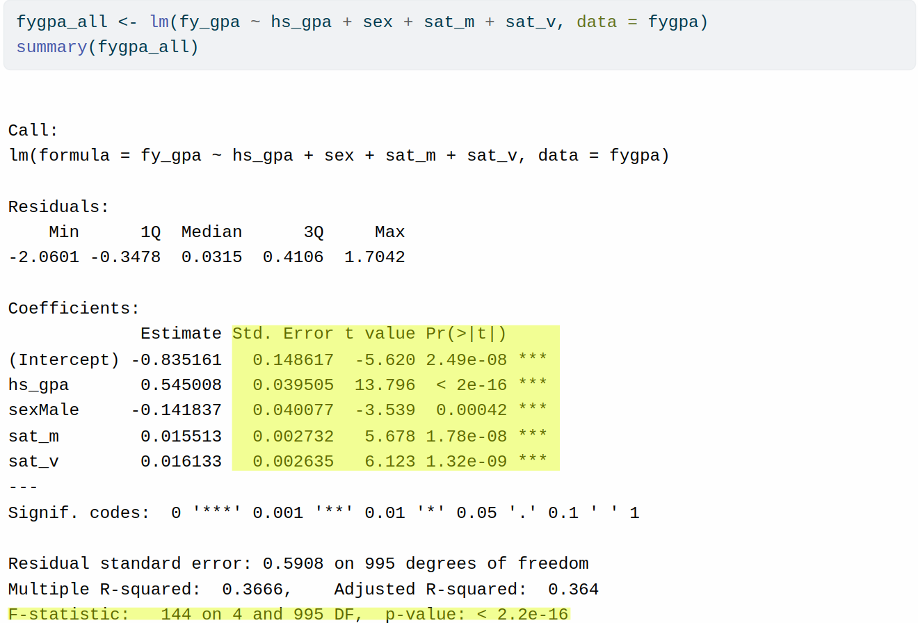
As we progress through this chapter we will learn what questions each of these tests tries to answer, as well as some other tests that are not available in the output of summary(). We will also learn how to construct (and interpret) confidence intervals for both the coefficients of the model and predictions.

8.3 The Working Assumptions

Just like for simple linear regression, inference for multiple linear regression is typically presented under a number of working assumptions; for the most part, we do not necessarily believe these assumptions are 100% true, but may be close enough to the truth that the inferences will still be useful.

Assumptions for Simple Linear Regression

Supose we observe dependent variables \(Y_i\) (\(i = 1,\ldots,N\)) and independent variables \(X_{ij}\) (\(i = 1,\ldots, N\) and \(j = 1,\ldots,P\)).

• Working Assumption 0 (“Full Rank”): None of the predictors can be perfectly predicted, in a linear fashion, from the other predictors. For example it is not possible to write \(X_{i1} = \alpha_0 + \alpha_1 \, X_{i2} + \cdots + \alpha_{P - 1} \, X_{iP}\) for some coefficients \((\alpha_0, \alpha_1, \ldots, \alpha_{P-1})\).

• Working Assumption 1 (“Linearity”): We can write \(Y_i = \beta_0 + \beta_1 \, X_{i1} + \cdots + \beta_P \, X_{iP} + \epsilon_i\) for some coefficients \(\beta_0, \ldots, \beta_P\) and error term \(\epsilon_i\). Additionally, we assume that the population average of the \(\epsilon_i\)’s is \(0\).

• Working Assumption 2 (Uncorrelated errors): The \(\epsilon_i\)’s are uncorrelated with each other.

• Working Assumption 3 (Constant Error Variance): The variance of the \(\epsilon_i\)’s is the same for all \(i\); we let \(\sigma^2\) be this common variance.

• Working Assumption 4 (Normality): The \(\epsilon_i\)’s are independent of each other and have a normal distribution, given \(X_1, \ldots, X_N\).

The assumptions are basically the same as for simple linear regression, with the exception of the full rank assumption. The full rank assumption essentially states that none of the independent variables in your model can be perfectly predicted by linearly regressing it onto the other variables; intuitively, this means that each predictor must contribute some unique information to the model.

To help understand this, here are some common situations in which the full rank assumption is often violated:

• For the GPA dataset, notice that we the variable sat_sum (the total SAT score) is available as a column, but has not been used. This is because it can be perfectly predicted from the variables sat_m and sat_v. If we had included sat_sum in the regression, we would actually run into problems because it is completely redundant. Exercise: try adding sat_sum in your regression; what happens when you look at the output of summary()?

• If you are using dummy variable for categorical predictors, including all possible categories violates this assumption. For example, if we are controlling for sex, with categories “male” and “female”, you only need on dummy variable rather than two. If you include both, you’ve created a perfect linear relationship (sexMale = 1 - sexFemale).

• The full rank assumption automatically fails when the number of independent variables \(P\) exceeds the sample size \(N\). This happens often, for example, in genomics, where \(P\) might correspond to gene expression levels for each gene you have and \(N\) might be relatively small.

In practice, violations of the full rank assumption are rare but can realistically occur.

8.4 Testing for Overall Significance of the Model

One issue that folks often try to address at the front of an analysis is whether there is any relationship between the dependent variable and any of the independent variables. I sometimes call this the “Am I Stupid?” test: if I somehow fail to (strongly) reject the null hypothesis, it sort of implies that I wasted my time collecting the data because I somehow managed to not capture any obvious relationships.

Formally, we consider the following null and alternative hypotheses:

• \(H_0\): \(\beta_1 = \beta_2 = \cdots = \beta_P = 0\); that is, all of the regression coefficients are zero.
• \(H_1\): At least one of the regression coefficients is non-zero.

Example: The GPA Dataset

In the context of the GPA dataset, the null hypothesis is that \(\beta_{\texttt{hs\_gpa}} = \beta_{\texttt{sat\_m}} = \beta_{\texttt{sat\_v}} = \beta_{\texttt{sex}} = 0\). In words, this states the high school GPA, the SAT scores, and sex are all unrelated to first year GPA.

To some extent, we already know that this null hypothesis is false, as we already showed in the section on inference for simple lienar regression that there is overwhelming evidence of a relationship between high school GPA and first year GPA.

In this section we will show how to test this null hypothesis using the overall \(F\)-test of model significance

8.4.1 The Regression and Error Sums of Squares

To understand the F-test for overall model significance, we first will re-introduce the sums of squares that we defined in Section 4.8.1, but now in the context of multivariate linear regression. Recall that the total, error, and regression sums of squares are given respectively by

\[ \begin{aligned} \text{SST} = \sum_i (Y_i - \bar Y)^2 \quad \text{SSE} = \sum_i (Y_i - \widehat Y_i)^2 \quad \text{and} \quad \text{SSR} = \sum_i (\widehat Y_i - \bar Y)^2. \end{aligned} \]

These sums of squares can be interpreted as follows:

• SST is the total amount of variability in the \(Y_i\)’s.
• SSR is the amount of variability in the \(Y_i\)’s that can be accounted for by the model.
• SSE is the amount of variability in the \(Y_i\)’s that cannot be accounted for by the model.

Each of these sums of squares is also associated with a certain number called its degrees of freedom. The degrees of freedom represent the number of independent pieces of information that go into the calculation of each sum of squares. Here’s an intuitive description of the number of degrees of freedom for each term:

• SST Degrees of Freedom (DFT): We start with \(N\) observations, but lose one degree of freedom ebcause we use the mean (\(\bar Y\)) in the calculation. Because of this, there are effectively on \(N - 1\) differences \((Y_i - \bar Y)\) that we are working with, because given \((Y_1 - \bar Y), \ldots, (Y_{N - 1} - \bar Y)\) we can do some algebra to work out \((Y_N - \bar Y)\). This reduces the number of pieces of information by \(1\). Accordingly there are \(\text{DFT} = N - 1\) degrees of freedom associated with SST.
• SSR Degrees of Freedom (DFR): We can compute the terms \((\widehat Y_i - \bar Y)\) using just the estimated regression coefficients \(\widehat \beta_0, \ldots, \widehat \beta_P\), which represent \(P + 1\) pieces of information. For a similar reason to SST, however, we lose one degree of freedom because we are using \(\bar Y\). Accordingly, there are \(\text{DFR} = P\) degrees of freedom associated with SSR.
• SSE Degrees of Freedom (DFE): We start with \(N\) observations, as with SST. Rather than just needing to use \(\bar Y\), however, we need to use \(\widehat \beta_0, \ldots, \widehat\beta_P\) i the calculation of SSE as well, causing us to lose \(P + 1\) degrees of freedom. Accordingly there are \(\text{DFE} = N - P - 1\) degrees of freedom associated with SSE.

8.4.2 Key Facts for the Sums of Squares

In addition to the definitions above, there are a couple of important facts that we will use to develop both the overall test for model significance as well as some other tests that we will develop later.

• Decomposition of Sums of Squares: The total variability is equal to the amount of variability accounted for by the model plus the amount of variabilty unaccounted for by the model: SST = SSR + SSE.
• Decomposition of Degrees of Freedom: The number of pieces of information needed to compute the total variability is equal to the number of pieces needed to compute the variability accounted for by the model plus the number of pieces to compute the variability unexplained by the model: DFT = DFR + DFE.

8.4.3 The F-test For Overall Model Significance

The \(F\)-test for overall model significance uses the test statistic

\[ F = \frac{\text{SSR} / P}{\text{SSE} / (N- P - 1)} \]

Under the null hypothesis that all of the regression coefficients are zero, this follows an \(F\)-distribution with \(P\) numerator degrees of freedom and \(N - P - 1\) denominator degrees of freedom. If the observed \(F\)-statistic is large, this suggests that at least one of the regression coefficients is non-zero, so we reject the null hypothesis that all \(\beta_j\)’s are zero. If instead the \(F\)-statistic is small, we fail to reject the null hypothesis.

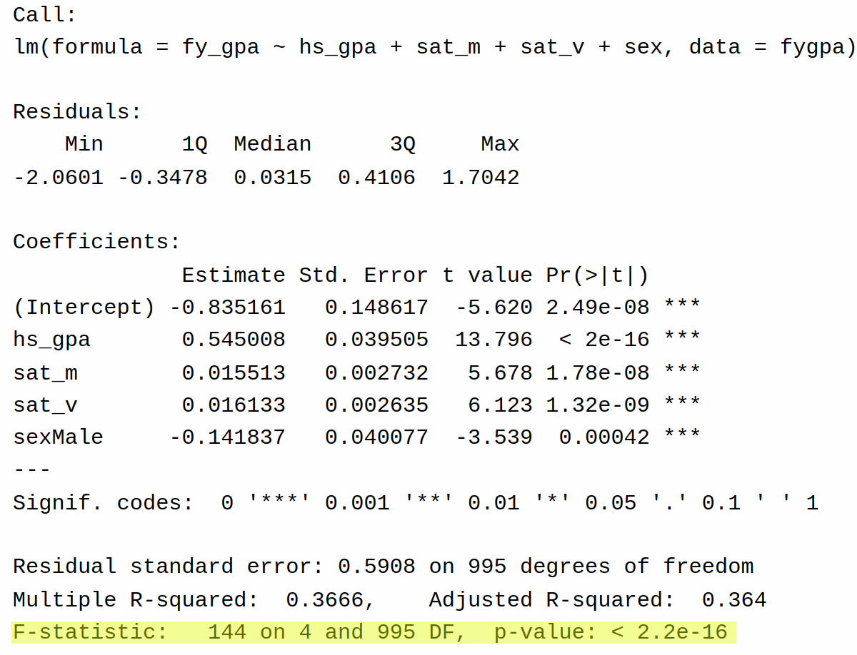
To see this in action, let’s revisit the output of summary() for the full model fit to the GPA dataset:

The same information is given by the output of glance() as well:

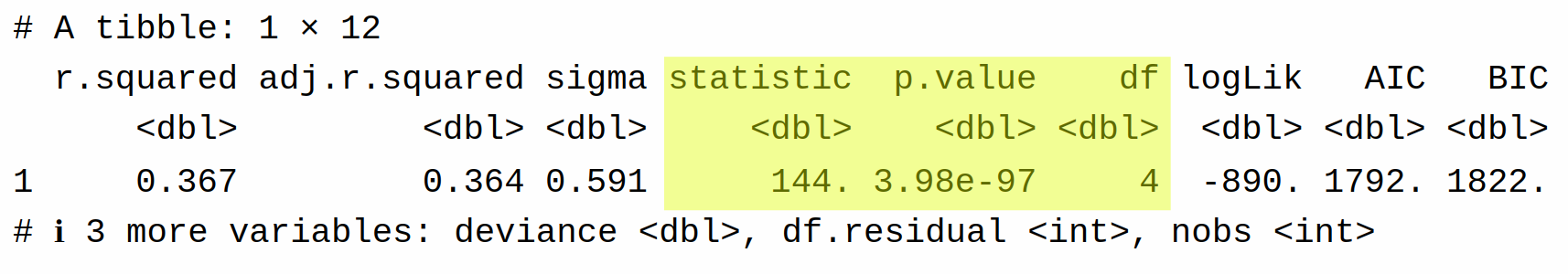
The relevant piece of this for us is the \(P\)-value less than \(2 \times 10^{-16} \approx 0\), indicating that there is very strong evidence that at least one of the (non-intercept) coefficients is non-zero. From this we can conclude that there is a relationship first year GPA and (at least one of) high school GPA, SAT math score, SAT verbal score, and sex.

8.4.4 More on the F Distribution

The \(F\)-distribution used above plays a central role in regression; not only is it used for the overall test of model significance, it will also be used to test more intricate hypotheses later.

The \(F\)-distribution is a continuous distribution (like the \(t\)-distribution and standard normal distribution) that takes only positive values. Like the \(t\)-distribution, it is characterized by degrees of freedom; unlike the \(t\)-distribution, there are actually two degrees of freedom, called the “numerator degrees of freedom” and “denominator degrees of freedom.” The terms come from the fact that \(F\)-statistics are usually a ratio of two quantities.

The figure below displays the density of the \(F\)-distribution for a variety of different numerator and denominator degrees of freedom:

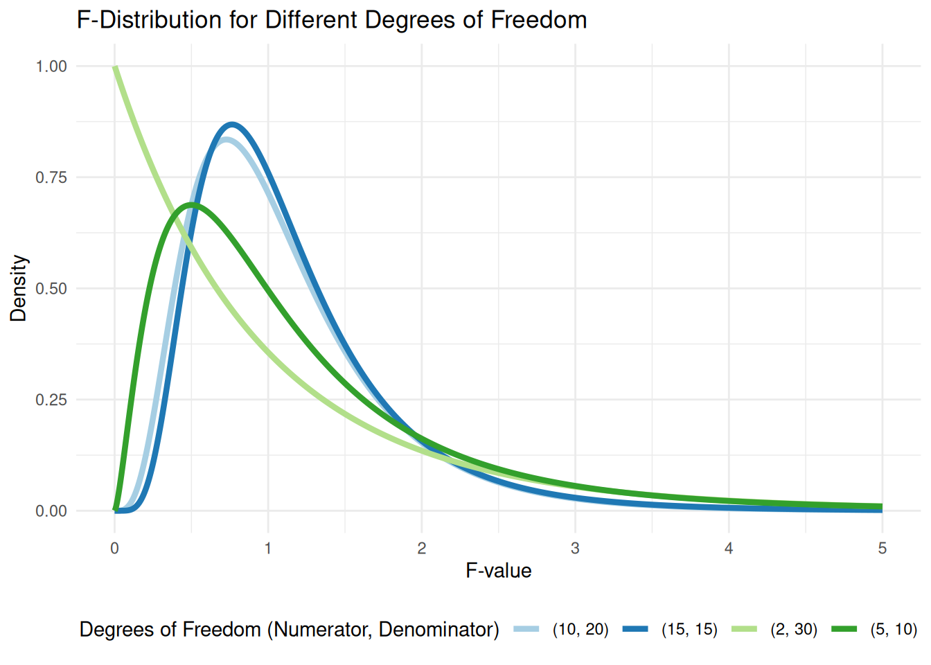
While \(T\)-statistics are generally “around 0” under the null hypothesis, \(F\)-statistics are generally “around 1.” The larger the denominator degrees of freedom. The F-distribution allows us to quantify the surprise of observing a given F-statistic under the null hypothesis. If the observed F-statistic is in the far right tail of the corresponding F-distribution, it suggests that the null hypothesis is unlikely to be true, leading us to reject it in favor of the alternative that at least one regression coefficient is non-zero.

8.4.5 The Relationship Between the F-test and R-Squared

There is an interesting connection between the \(F\)-statistic for testing overall model significance and multiple R-squared. Recall that \(R^2\) is defined as

\[ R^2 = \frac{\text{SSR}}{\text{SST}} = 1 - \frac{\text{SSE}}{\text{SST}}. \]

Plugging this into the \(F\)-statistic formula, we can rewrite it as

\[ F = \frac{R^2}{1 - R^2} \times \frac{N - P - 1}{P}. \]

This can be verified by the output on the GPA dataset. From the output of summary, we have \(R^2 = 0.367\), \(P = 4\), and \(N - P - 1 = 995\), giving

0.367 / (1 - 0.367) * 995 / 4

[1] 144.22

which agrees with the formula we saw above.

Why this matters: This formula provides an intuitive interpretation of the \(F\)-test. The first term \(R^2 / (1 - R^2)\) is large if the predictors account for a lot of the variability in the data: better \(R^2\), bigger \(F\)-statistic. The second term \((N - P - 1) / P\) is a term that gets bigger the larger the sample size: even if \(R^2\) is small, we can still get a large \(F\)-statistic if our sample size is large. Conversely, the more predictors we try to control for the smaller \((N - P - 1) / P\) will be, so if we try to control for too many things that do not increase \(R^2\) we will end up making it harder to figure out that a relationship exists.

8.5 Hypothesis Testing and Confidence Intervals for Individual Coefficients

A couple of common questions when working with a linear regression model are:

1. Is there evidence that one of the independent variables (say, sex in the GPA example) is unrelated to the dependent variable, after accounting for the other independent variables?

2. The coefficient estimate \(\beta_j\) represents the average change in the dependent variable given a unit change in \(X_{ij}\) after accounting for the other independent variables; what are a plausible range of values for this change?

We can address these questions using the familiar tools of hypothesis testing and confidence intervals.

8.5.1 Null and Alternative Hypotheses

For a particular coefficient of interest \(\beta_j\), we typically test the following hypotheses:

• \(H_0: \beta_j = 0\) (The predictor \(X_j\) has no effect on \(Y\) when controlling for other predictors)
• \(H_1: \beta_j \neq 0\) (The predictor \(X_j\) has some effect on \(Y\) when controlling for other predictors)

For a concrete example, we might test the null hypothesis \(H_0: \beta_{\texttt{sex}} = 0\) in the GPA example to determine whether men and women, who are otherwise identical in terms of SAT scores and high school GPA, tend to perform differently in their first year. Sometimes, we might also be interested in testing whether a coefficient is equal to some other value, or in one-sided tests (e.g., \(H_0: \beta_{\texttt{sex}} > 0\), which would correspond to the statement that men tend to do better than women in their first year all other things being equal), but the above is the most common formulation.

8.5.2 T-Statistics and P-Values

To test these hypotheses, we use a \(T\)-statistic. The \(T\)-statistics and \(P\)-values for the least squares estimators in multiple regression take the same form as they do in simple linear regression. The \(T\)-statistic is given by

\[ T_{\widehat\beta_j} = \frac{\widehat\beta_j}{s_{\widehat\beta_j}} \]

where \(s_{\widehat\beta_j}\) is the standard error of \(\widehat\beta_j\). The standard error for each coefficient is in the output here:

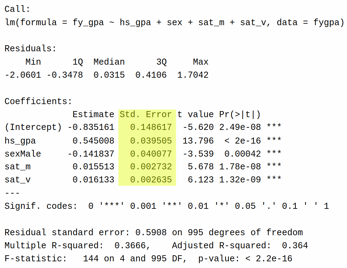
Under the null hypothesis, this t-statistic follows a t-distribution with \(N - P - 1\) degrees of freedom, where \(N\) is the number of observations and \(P\) is the number of predictors (excluding the intercept). The p-value is then calculated as the probability of observing a \(T\)-statistic as extreme as or more extreme than the one calculated, assuming the null hypothesis is true.

Based on the above table (specifically, that all of the \(P\)-values are close to zero) we can conclude the following:

1. There is very strong evidence that high school GPA is significantly associated with first-year college GPA, controlling for other factors in the model.

2. There is strong evidence of a significant difference in first-year GPA between males and females, controlling for other factors. The negative test statistic suggests that, on average, males tend to have lower first-year GPAs than females.

3. There is very strong evidence that SAT math scores are significantly associated with first-year college GPA, controlling for other factors.

4. The high school GPA seems to have the strongest association with first-year college GPA, followed by SAT verbal and math scores.

Optional: Standard Errors for the Regression Coefficients

Just like the least squares estimators have a more complicated form when dealing with multiple linear regression, the standard errors are also more complicated. Convenient formulas can only be given in terms of matrix algebra. Specifically, the standard error of \(\widehat \beta_j\) is given by

\[ s_{\widehat\beta_j} = \sqrt{s \, (\mathbf X^\top \mathbf X)_{jj}^{-1}} \]

where \((\mathbf X^\top \mathbf X)^{-1}_{jj}\) denotes the \((j,j)\)th entry of the matrix \((\mathbf X^\top \mathbf X)^{-1}\).

8.5.3 Confidence Intervals

Confidence intervals for regression coefficients in multiple linear regression are conceptually similar to those in simple linear regression. They provide a range of plausible values for the true population parameter, given our sample data and model assumptions.

For a particular coefficient \(\beta_j\), a \(100(1-\alpha)\%\) confidence interval is given by:

\[ \beta_j = \widehat{\beta}_j \pm t_{\alpha/2} \cdot s_{\widehat{\beta}_j} \]

Where:

• \(\widehat{\beta}_j\) is the estimated coefficient
• \(t_{\alpha/2}\) is the critical value from the \(t\)-distribution with \(N - P - 1\) degrees of freedom
• \(s_{\widehat{\beta}_j}\) is the standard error of the coefficient estimate
• \(N\)is the number of observations
• \(P\) is the number of coefficients in the model (excluding the intercept)

The confidence interval has the usual interpretation: assuming that our working assumptions hold, if we were to repeat our sampling process many times and construct this interval each time, approximately \(100(1 - \alpha)\%\) of the time the interval will contain the true value of the parameter. In shorthand, we say that we are \(100(1-\alpha)\%\) confident that the true value of \(\beta_j\) lies within our confidence interval.

Let’s construct a 95% confidence interval for the coefficient of high school GPA in our multiple regression model. In R we can do this using the confint() function:

confint(fygpa_all, "hs_gpa", level = 0.95)

           2.5 %   97.5 %
hs_gpa 0.4674857 0.622531

We can interpret this as follows:

1. we are 95% confident that
2. given two populations students who are otherwise identical (same sex and same SAT scores) who have high school GPAs that differ by 1 grade point
3. the population average first year GPAs differ by between 0.47 and 0.62.

(If you want all of the confidence intervals for the coefficients in the model then you can omit the argument "hs_gpa".)

8.6 Confidence and Prediction Intervals for Predictions

In addition to making point predictions, it’s often useful to quantify the uncertainty associated with these predictions. We can do this using confidence intervals and prediction intervals. These intervals are interpreted in the same way that they are for simple linear regression.

A confidence interval for the mean prediction provides a range of plausible values for the average response (Y) for a given set of predictor values (X). It represents the uncertainty in estimating the population mean. For a new set of independent variables \(X_{01}, \ldots, X_{0P}\) we can construct a \(100(1-\alpha)\%\) confidence interval for the mean predict as

\[ \widehat Y_0 \pm t_{\alpha/2} \times s_{\widehat Y_{0}} \]

where \(\widehat Y_0\) is the predicted value for the new observation, \(s_{\widehat Y_0}\) is its standard error, and \(t_{\alpha/2}\) is the relevant critical value from the \(t\)-distribution with \(N - P - 1\) degrees of freedom.

Optional: A Formula for the Standard Error

The standard error of the prediction is calculated as:

\[ s_{\widehat Y_0} = s \times \sqrt{\mathbf H_{ii}} \qquad \text{where} \qquad \mathbf H = \mathbf X (\mathbf X^\top \mathbf X)^{-1} \mathbf X^\top \]

where \(s\) is the residual standard error and \(\mathbf H\) is called the “hat matrix”. The hat matrix gets its name from the fact that \(\mathbf H \mathbf Y = \widehat{\mathbf Y}\) where \(\widehat{\mathbf Y} = (\widehat Y_1, \ldots, \widehat Y_N)\) so that \(\mathbf H\) “puts the hat on” \(\mathbf Y\).

Prediction intervals, on the other hand, provide a range of a plausible values for an individual new observation, rather than the mean. It accounts for both the uncertainty in estimating the mean and the variability of individual observations around the mean. The prediction interval is instead given by

\[ \widehat Y_0 \pm t_{\alpha/2} \sqrt{s^2 + s^2_{\widehat Y_0}}. \]

The prediction interval is always wider than the confidence interval for the same set of predictor values, as it accounts for additional uncertainty.

8.6.1 Example: GPA Dataset

We can create confidence and prediction intervals for each of the observations in our dataset using the predict() function:

## Confidence intervals for each observation in the dataset
predict(fygpa_all, interval = "confidence")

## predictions intervals for each observation in the dataset
predict(fygpa_all, interval = "prediction")

or by using the augment() function:

augment(fygpa_all, interval = "confidence")

# A tibble: 1,000 × 13
   fy_gpa hs_gpa sex    sat_m sat_v .fitted .lower .upper  .resid    .hat .sigma
    <dbl>  <dbl> <chr>  <int> <int>   <dbl>  <dbl>  <dbl>   <dbl>   <dbl>  <dbl>
 1   3.18   3.4  Male      62    65    2.89   2.80   2.97  0.293  0.00569  0.591
 2   3.33   4    Female    64    58    3.27   3.19   3.35  0.0566 0.00493  0.591
 3   3.25   3.75 Female    60    56    3.04   2.98   3.11  0.207  0.00342  0.591
 4   2.42   3.75 Male      53    42    2.57   2.48   2.65 -0.147  0.00559  0.591
 5   2.63   4    Male      52    55    2.90   2.80   2.99 -0.267  0.00698  0.591
 6   2.91   4    Female    56    55    3.10   3.03   3.17 -0.191  0.00405  0.591
 7   2.83   2.8  Male      65    57    2.48   2.40   2.56  0.353  0.00499  0.591
 8   2.51   3.8  Male      62    53    2.91   2.84   2.98 -0.401  0.00355  0.591
 9   3.82   4    Female    77    67    3.62   3.49   3.75  0.200  0.0121   0.591
10   2.54   2.6  Male      44    41    1.78   1.71   1.86  0.756  0.00445  0.591
# ℹ 990 more rows
# ℹ 2 more variables: .cooksd <dbl>, .std.resid <dbl>

augment(fygpa_all, interval = "prediction")

# A tibble: 1,000 × 13
   fy_gpa hs_gpa sex    sat_m sat_v .fitted .lower .upper  .resid    .hat .sigma
    <dbl>  <dbl> <chr>  <int> <int>   <dbl>  <dbl>  <dbl>   <dbl>   <dbl>  <dbl>
 1   3.18   3.4  Male      62    65    2.89  1.72    4.05  0.293  0.00569  0.591
 2   3.33   4    Female    64    58    3.27  2.11    4.44  0.0566 0.00493  0.591
 3   3.25   3.75 Female    60    56    3.04  1.88    4.20  0.207  0.00342  0.591
 4   2.42   3.75 Male      53    42    2.57  1.40    3.73 -0.147  0.00559  0.591
 5   2.63   4    Male      52    55    2.90  1.73    4.06 -0.267  0.00698  0.591
 6   2.91   4    Female    56    55    3.10  1.94    4.26 -0.191  0.00405  0.591
 7   2.83   2.8  Male      65    57    2.48  1.31    3.64  0.353  0.00499  0.591
 8   2.51   3.8  Male      62    53    2.91  1.75    4.07 -0.401  0.00355  0.591
 9   3.82   4    Female    77    67    3.62  2.45    4.79  0.200  0.0121   0.591
10   2.54   2.6  Male      44    41    1.78  0.622   2.95  0.756  0.00445  0.591
# ℹ 990 more rows
# ℹ 2 more variables: .cooksd <dbl>, .std.resid <dbl>

For both outputs of the augment() function the lower endpoint and upper endpoint are given by .lower and .upper.

Some examples of what we can read off from these outputs are given below:

• The first row corresponds to a male student with a high school GPA of 3.4, SAT verbal score of 650, and SAT math score of 620. The results for the confidence interval states that we are 95% confident that the average first-year GPA for all students with these characteristics are between 2.80 and 2.97. For the prediction interval we are 95% confident that for a single student with these characteristics their GPA will be between 1.72 and 4.05.
• The second row corresponds to a female student with a high school GPA of 4.0, SAT verbal score of 580, and SAT math score of 640. The results for the confidence interval states that we are 95% confident that the average first-year GPA for all students with these characteristics is between 3.19 and 3.35. For the prediction interval we are 95% confident that for a single student with these characteristics their GPA will be between 2.11 and 4.44.

Again, notice that the confidence intervals are always narrower than the prediction variables for each student. This is because confidence intervals estimate the mean response in a given subpopulation, while prediction intervals also account for individual variability.

8.7 Nested Model Comparisons Using F-Tests

In addition to testing for the overall model significance, we often want to compare two models, one simpler model and one more complex model, in order to determine if the more complex model is required or if the simpler model suffices. We have already done this to some extent with our tests for whether a given coefficient \(\beta_j\) in a model is zero or not (corresponding to a model that either excludes the variable \(X_{ij}\) or includes it).

Let’s be a bit more concrete: for the GPA dataset, we might want to know whether the SAT scores (sat_m and sat_v) lead to better predictions of GPA. So, we might want to compare a simple model

\[ \texttt{fy\_gpa}_i = \beta_0 + \beta_{\texttt{sex}} \, \texttt{sex}_i + \beta_{\texttt{hs\_gpa}} \, \texttt{hs\_gpa} + \epsilon_i \]

to a more complex model

\[ \texttt{fy\_gpa}_i = \beta_0 + \beta_{\texttt{sex}} \, \texttt{sex}_i + \beta_{\texttt{hs\_gpa}} \, \texttt{hs\_gpa} + \beta_{\texttt{sat\_m}} \, \texttt{sat\_m} + \beta_{\texttt{sat\_v}} \, \texttt{sat\_v} + \epsilon_i \]

In this case, we are interested in a test for whether two of the coefficients are equal to zero. Specifically, we want to test

• \(H_0\): both \(\beta_{\texttt{sat\_m}}\) and \(\beta_{\texttt{sat\_v}}\) are equal to zero.
• \(H_1\): at least one of \(\beta_{\texttt{sat\_m}}\) and \(\beta_{\texttt{sat\_v}}\) is not equal to zero.

To appropriate tool for doing this assessment is the \(F\)-test of nested models, which we describe below.

8.7.1 Sums of Squares for Nested Models

Let’s say we have two models:

• A reduced model that contains only \(Q\) non-intercept coefficients. For the GPA dataset, this would be the model that only includes sex and high school GPA as independent variables, so \(Q = 2\).
• A full model that contains \(P\) non-intercept coefficients. For the GPA dataset, this would be the model that includes sex, high school GPA, and both SAT scores, so \(P = 4\).

Because the full model contains all the terms in the reduced model, intuitively we should expect that the full model accounts for more variability in the outcome than the reduced model, i.e.,

\[ \text{SSR}_{\text{full}} \ge \text{SSR}_{\text{reduced}}, \]

where the SSRs are the regression sum of squares for the full and reduced models. This is true even if the reduced model is correct! The question is whether the improvement in fit of the full model is large enough to believe that the reduced model is incorrect. For the GPA dataset, for example, the question is whether including the SAT scores increase amount of variability accounted for by the regression a large amount (so that we believe they are required) or only a little bit (which happens even if they are not required).

8.7.2 The F-Test for Testing Nested Models

In terms of null and alternative hypotheses, we can frame things as follows:

• \(H_0\): the reduced model is correct.
• \(H_1\): the reduced model is not correct.

The \(F\)-test to test the above null/alternative hypothesis uses the \(F\)-statistic:

\[ F = \frac{\text{SSR}_{\text{full}} - \text{SSR}_{\text{reduced}}}{\text{SSE}_{\text{full}}} \times \frac{N - P - 1}{P - Q} \]

Under the null hypothesis that the additional predictors in the full model are not needed, it can be shown that this \(F\)-statistic follows an \(F\)-distribution with \(P - Q\) numerator degrees of freedom and \(N - P - 1\) denominator degrees of freedom.

Just like with the \(F\)-test for overall model significance, if the observed \(F\)-statistic is large, this is evidence against \(H_0\). If the \(F\)-statistic is small, we instead fail to reject the null hypothesis.

8.7.3 Testing Nested Hypotheses Using anova()

We can implement the test of nested models using the anova() function in R. To do this, we need to fit both the reduced model and the full model, and then plug these models into the function. For the GPA dataset, we have

fygpa_reduced <- lm(fy_gpa ~ hs_gpa + sex, data = fygpa)
fygpa_full <- lm(fy_gpa ~ hs_gpa + sex + sat_m + sat_v, data = fygpa)

anova(fygpa_reduced, fygpa_all)

Analysis of Variance Table

Model 1: fy_gpa ~ hs_gpa + sex
Model 2: fy_gpa ~ hs_gpa + sex + sat_m + sat_v
  Res.Df    RSS Df Sum of Sq      F    Pr(>F)    
1    997 386.07                                  
2    995 347.26  2    38.812 55.603 < 2.2e-16 ***
---
Signif. codes:  0 '***' 0.001 '**' 0.01 '*' 0.05 '.' 0.1 ' ' 1

I recommend instead looking at the tidy’d version of this:

tidy(anova(fygpa_reduced, fygpa_all))

# A tibble: 2 × 7
  term                         df.residual   rss    df sumsq statistic   p.value
  <chr>                              <dbl> <dbl> <dbl> <dbl>     <dbl>     <dbl>
1 fy_gpa ~ hs_gpa + sex                997  386.    NA  NA        NA   NA       
2 fy_gpa ~ hs_gpa + sex + sat…         995  347.     2  38.8      55.6  1.28e-23

The two rows in this table represent (1) the reduced model and (2) the full model. The columns of the table represent:

• term: A description of the model comparison being performed.

  • The first row shows the formula for the reduced model (fy_gpa ~ hs_gpa + sex).
  • The second row shows the formula for the full model (fy_gpa ~ hs_gpa + sat_m + sat_v + sex).

• df.residual: The residual degrees of freedom for each model, i.e., \(N\) (1000) minus the number of coefficients.

  • For the base model, we have \(2\) coefficients for the sex and high school GPA, as well as the intercept, so \(1000 - 3 = 997\).
  • For the full model, it’s \(995\), as we also have two more coefficients for the SAT scores.

• rss: The residual sum of squares (SSE) for each model.

  • For the reduced model, SSE is 386.
  • For the full model, SSE is 347.

• df: The difference in degrees of freedom between the two models, which is 2 in this case. This gives the numerator degrees of freedom for the \(F\)-test, as \(P = 4\) and \(Q = 2\).

• sumsq: The quantity \(\text{SSR}_{\text{full}} - \text{SSR}_{\text{reduced}}\). This also happens to be equal to \(\text{SSE}_{\text{reduced}} - \text{SSE}_{\text{full}}\), so we get 386.07 - 347.26 \(\approx\) 38.8.

• statistic: The F-statistic for testing the null hypothesis, calculated as:

  \[ F = \frac{38.8}{347.2} \times \frac{995}{2} = 55.6 \]

• p.value: The p-value associated with the F-statistic. The very small p-value (1.28e-23) suggests that the additional predictors in the full model (sat_m and sat_v) do indeed have significant explanatory power.

8.7.4 Sequential Tests Using anova()

When applied to a single model, the anova() functin performs a series of tests called sequential \(F\)-tests. These tests compare nested models in a specific order, determined by the order in which the predictors are added to the model. This approach allows us to assess the incremental contribution of each predictor to the model.

Let’s examine the output of anova() for our full model:

anova(fygpa_all)

Analysis of Variance Table

Response: fy_gpa
           Df Sum Sq Mean Sq  F value    Pr(>F)    
hs_gpa      1 161.86 161.860 463.7743 < 2.2e-16 ***
sex         1   0.31   0.312   0.8945    0.3445    
sat_m       1  25.73  25.726  73.7123 < 2.2e-16 ***
sat_v       1  13.09  13.086  37.4943 1.318e-09 ***
Residuals 995 347.26   0.349                       
---
Signif. codes:  0 '***' 0.001 '**' 0.01 '*' 0.05 '.' 0.1 ' ' 1

We can also look at the tidy’d version:

tidy(anova(fygpa_all))

# A tibble: 5 × 6
  term         df   sumsq  meansq statistic   p.value
  <chr>     <int>   <dbl>   <dbl>     <dbl>     <dbl>
1 hs_gpa        1 162.    162.      464.     9.63e-85
2 sex           1   0.312   0.312     0.895  3.44e- 1
3 sat_m         1  25.7    25.7      73.7    3.44e-17
4 sat_v         1  13.1    13.1      37.5    1.32e- 9
5 Residuals   995 347.      0.349    NA     NA       

For each row in the above table, the null hypothesis being tested is:

• \(H_0\): the coefficient(s) associated to this variable are all equal to \(0\), given that all predictors given above it are already included in the model (but none below it).
• \(H_1\): at least one of the coefficient(s) associated to this variable are not equal to zero, given that all predictors above it are included in the model (but none below it).

More specifically:

1. hs_gpa: Tests whether high school GPA improves the model compared to an intercept-only model. That is, it tests the model fy_gpa ~ hs_gpa as the alternative, relative to a null model that does not control for any of the independent variables.

2. sex: Tests whether sex improves the model that already includes high school GPA. It tests the null model fy_gpa ~ hs_gpa against the alternative fy_gpa ~ hs_gpa + sex.

3. sat_m: Tests whether SAT math scores improve the model that already includes high school GPA and sex. It tests the null model fy_gpa ~ hs_gpa + sex against the alternative fy_gpa ~ hs_gpa + sex + sat_m.

4. sat_v: Tests whether SAT verbal scores improve the model that already includes high school GPA, sex, and SAT math scores. It tests the null model fy_gpa ~ hs_gpa + sex + sat_m against the alternative fy_gpa ~ hs_gpa + sex + sat_m + sat_v.

Warning

Note that the order in which the variables appear in the formula statement matters, as this determines which tests will be done! For example, fitting a model with fy_gpa ~ hs_gpa + sex will give different sequential tests than if we fit a model with fy_gpa ~ sex + hs_gpa. Exercise: Which tests would each of these alternatives do?

The specific columns of the output correspond to the following:

1. term: This column lists the variables in the order they were added to the model, plus the residuals.

2. df: Degrees of freedom.

   • For each independent variable, the degrees of freedom is the number of coefficients associated to that variable (so 1 for these particular sets, but if we are looking at non-numeric variables we would have to count all of the dummy variables associated to the variable)
   • For the residuals, it’s 995, which is the sample size (1000) minus the number of coefficients in the full model (four variables plus an additional 1 for the intercept).

3. sumsq: Sum of Squares.

   • For predictors, this is the reduction in the error sum of squares when the term is added to the model.
   • For residuals, this is the remaining unexplained variance.

4. meansq: Mean Square. This is the Sum of Squares divided by the degrees of freedom.

   • For predictors, it represents the average reduction in error variance per degree of freedom.
   • For residuals, it’s an estimate of the error variance (\(\sigma^2\)).

5. statistic: The F-statistic for each predictor.

   • Calculated as (predictor’s Mean Square) / (Residual Mean Square).
   • Not applicable (NA) for the residuals row.

6. p.value: The p-value associated with each F-statistic. Not applicable (NA) for the residuals row.

Interpreting the output, we observe the following:

• High school GPA has a very small \(P\)-value, indicating that including it improves upon the intercept-only model.
• Sex has a large \(P\)-value, suggesting that there is no evidence that it improves the model relative to a model that includes only high school GPA.
• Both SAT math and SAT verbal scores have and very small p-values, indicating they significantly improve the model even after accounting for high school GPA and sex (and SAT math in the case of SAT verbal).
• The residuals row shows that, on average, the predictions of the full model are off by around \(\sqrt{0.349} \approx 0.59\) grade points on average.

8.7.5 Single Term Deletion Tests

While sequential tests assess the contribution of each variable in a specific order, single term deletion tests provide a different perspective. These tests, performed using the drop1() function in R, evaluate the significance of each predictor by comparing the full model to a model where that predictor is removed, keeping all other predictors in place.

Comparison to the Output of Summary

What is being tested here is almost exactly the same thing as what is being tested by the code summary(fygpa_all): that the coefficient associated to each independent variable is zero. The only difference between the drop1() tests and the output of summary() is in how non-numeric variables are handled; drop1() tests all coefficients of a non-numeric variable simultaneously rather testing the coefficients individually.

Let’s examine the output of drop1() for our full model:

drop1(fygpa_all, test = "F")

Single term deletions

Model:
fy_gpa ~ hs_gpa + sex + sat_m + sat_v
       Df Sum of Sq    RSS      AIC F value    Pr(>F)    
<none>              347.26 -1047.68                      
hs_gpa  1    66.425 413.69  -874.65 190.328 < 2.2e-16 ***
sex     1     4.371 351.63 -1037.17  12.525 0.0004201 ***
sat_m   1    11.254 358.51 -1017.79  32.245 1.783e-08 ***
sat_v   1    13.086 360.35 -1012.69  37.494 1.318e-09 ***
---
Signif. codes:  0 '***' 0.001 '**' 0.01 '*' 0.05 '.' 0.1 ' ' 1

For each predictor in the table, the null hypothesis being tested is:

• \(H_0\): The coefficients associated with this predictor is equal to 0, given that all other predictors are in the model.
• \(H_1\): The coefficients associated with this predictor is not equal to 0, given that all other predictors are in the model.

More specifically:

1. hs_gpa: Tests whether high school GPA improves the model that already includes sex, SAT math, and SAT verbal scores. It tests the null model fy_gpa ~ sex + sat_m + sat_v against the alternative fy_gpa ~ hs_gpa + sex + sat_m + sat_v.

2. sex: Tests whether sex improves the model that already includes high school GPA, SAT math, and SAT verbal scores. It tests the null model fy_gpa ~ hs_gpa + sat_m + sat_v against the alternative fy_gpa ~ hs_gpa + sex + sat_m + sat_v.

3. sat_m: Tests whether SAT math scores improve the model that already includes high school GPA, sex, and SAT verbal scores. It tests the null model fy_gpa ~ hs_gpa + sex + sat_v against the alternative fy_gpa ~ hs_gpa + sex + sat_m + sat_v.

4. sat_v: Tests whether SAT verbal scores improve the model that already includes high school GPA, sex, and SAT math scores. It tests the null model fy_gpa ~ hs_gpa + sex + sat_m against the alternative fy_gpa ~ hs_gpa + sex + sat_m + sat_v.

The specific columns of the output correspond to the following:

1. term: This column lists the variables being tested for deletion, plus <none> which represents the full model.

2. df: Degrees of freedom associated with each term (1 for each predictor in this case).

3. sumsq: Sum of Squares. This is the increase in the error sum of squares if the term is dropped from the model.

4. rss: Residual Sum of Squares for the model after dropping the term.

5. AIC: Akaike Information Criterion for the model after dropping the term. Ignore this for now, we will learn about AIC later.

6. statistic: The F-statistic for testing whether the term can be dropped.

7. p.value: The p-value associated with each F-statistic.

Interpreting the output, we observe the following:

• High school GPA, SAT math, and SAT verbal scores are all statistically significant, as they were with the sequential tests; the difference is that they are all significant assuming all other variables are already included in the model.
• Sex is also significant, with a \(P\)-value less than 0.001.
• All of these \(P\)-values agree exactly with the output of summary.

Comparison with Sequential Tests

Note that unlike in the sequential tests, where sex appeared non-significant, in the single term deletion tests, sex is shown to be a significant predictor (p = 0.0004201) when controlling for all other variables. This highlights an important distinction: the significance of a predictor can depend on which other predictors are in the model and the order in which they are added.

To see a setting where we actually get different results than summary(), we can look at the iris dataset:

data(iris)
head(iris)

  Sepal.Length Sepal.Width Petal.Length Petal.Width Species
1          5.1         3.5          1.4         0.2  setosa
2          4.9         3.0          1.4         0.2  setosa
3          4.7         3.2          1.3         0.2  setosa
4          4.6         3.1          1.5         0.2  setosa
5          5.0         3.6          1.4         0.2  setosa
6          5.4         3.9          1.7         0.4  setosa

We have already looked at this dataset before, so run ?iris if you want a quick refreshed. Now, let’s consider predicting Sepal.Length using all of the other variables:

iris_lm <- lm(Sepal.Length ~ Sepal.Width + Petal.Length + 
                Petal.Width + Species, data = iris)
summary(iris_lm)

Call:
lm(formula = Sepal.Length ~ Sepal.Width + Petal.Length + Petal.Width + 
    Species, data = iris)

Residuals:
     Min       1Q   Median       3Q      Max 
-0.79424 -0.21874  0.00899  0.20255  0.73103 

Coefficients:
                  Estimate Std. Error t value Pr(>|t|)    
(Intercept)        2.17127    0.27979   7.760 1.43e-12 ***
Sepal.Width        0.49589    0.08607   5.761 4.87e-08 ***
Petal.Length       0.82924    0.06853  12.101  < 2e-16 ***
Petal.Width       -0.31516    0.15120  -2.084  0.03889 *  
Speciesversicolor -0.72356    0.24017  -3.013  0.00306 ** 
Speciesvirginica  -1.02350    0.33373  -3.067  0.00258 ** 
---
Signif. codes:  0 '***' 0.001 '**' 0.01 '*' 0.05 '.' 0.1 ' ' 1

Residual standard error: 0.3068 on 144 degrees of freedom
Multiple R-squared:  0.8673,    Adjusted R-squared:  0.8627 
F-statistic: 188.3 on 5 and 144 DF,  p-value: < 2.2e-16

There are now two coefficients associated with Species. However, if we run drop1() we get

drop1(iris_lm, test = "F")

Single term deletions

Model:
Sepal.Length ~ Sepal.Width + Petal.Length + Petal.Width + Species
             Df Sum of Sq    RSS     AIC  F value    Pr(>F)    
<none>                    13.556 -348.57                       
Sepal.Width   1    3.1250 16.681 -319.45  33.1945 4.868e-08 ***
Petal.Length  1   13.7853 27.342 -245.33 146.4310 < 2.2e-16 ***
Petal.Width   1    0.4090 13.966 -346.11   4.3448   0.03889 *  
Species       2    0.8889 14.445 -343.04   4.7212   0.01033 *  
---
Signif. codes:  0 '***' 0.001 '**' 0.01 '*' 0.05 '.' 0.1 ' ' 1

We now see that there is a single row associated to Species that has two degrees of freedom. The difference between the tests being conducted is:

• In summary(), we have separate tests for \(\beta_{\text{Speciesvirginica}} = 0\) and \(\beta_{\text{Speciesversicolor}} = 0\).
• In drop1(), we have a single test for \(\beta_{\text{Speciesvirginica}} = \beta_{\text{Speciesversicolor}} = 0\).

Practical Guidance

Generally, for non-numeric predictors, you are going to want to test for the coefficients of that predictor simultaneously. Usually if we think that one coefficient for a non-numeric variable is non-zero, we probably think that they all should be. This is not always the case, but it is the case much more often than not.

8.7.6 Choosing Between Single Term Deletion and Sequential Tests

Both single term deletion tests and sequential tests are valuable tools in multiple regression analysis, but they serve different purposes and are appropriate in different situations.

Single term deletion tests are useful when one or more of the following are true:

• You want to assess the significance of each predictor after controlling for all of the others.
• The predictors have no natural ordering.

Sequential tests are useful when:

• You have a theoretical basis for the order of the predictors. For example, you might want to know if SAT scores improve upon high school GPA because GPA does not require individuals to take a standardized test.

• In studies where the variables have a natural hierarchy, sequential tests reflect this structure; we will see this in later chapters when we consider the two topics of interaction effects and polynomial regression.

Again, it’s important to remember that sequential and single-term deletion tests can give different results. A predictor might be significant in a single term deletion test but not in a sequential test (or vice versa), depending on the other predictors in the model and their order.

8.8 Exercises

8.8.1 Exercise 1: Boston Housing, Again

Using the Boston Housing dataset once again

Boston <- MASS::Boston

predicting medv using rm, lstat, crim, and nox, perform the following analyses:

a, Conduct an F-test for overall model significance. What is your conclusion about the model’s overall explanatory power?

b, Perform t-tests for each coefficient in the model. Which predictors are statistically significant at the 0.05 level? Interpret the p-values in the context of the problem.

3. Construct and interpret 95% confidence intervals for each coefficient. Interpret the coefficient for nox in terms of the effect of a unit increase in nox on medv.

4. Use the predict() function to calculate a 95% prediction interval for the median home value in a tract with 6 average rooms, 8% lower status individuals, a crime rate of 0.22, and nitric oxide concentration of 0.585. Interpret this interval in the context of the problem.

5. Fit a reduced model that only includes rm and lstat as predictors. Use an F-test to compare this reduced model to the full model from the previous exercise. What do you conclude about the importance of including crim and nox in the model? State carefully the null and alternative hypotheses, and whether the null can be rejected.

6. Perform a sequential ANOVA using the anova() function on the full model, with predictors entered in the order: nox, lstat, crim, rm. Interpret the results for each predictor. How might these results change if you altered the order of the predictors?

8.8.2 Exercise 2: Affairs Revisited

This exercise revisits the Affairs dataset to look at multiple factors and see to what extent they predict the occurence of extra-marital affairs. First, load the data by running

library(AER)

Loading required package: car

Loading required package: carData

Attaching package: 'car'

The following object is masked from 'package:dplyr':

    recode

The following object is masked from 'package:purrr':

    some

Loading required package: lmtest

Loading required package: zoo

Attaching package: 'zoo'

The following objects are masked from 'package:base':

    as.Date, as.Date.numeric

Loading required package: sandwich

Loading required package: survival

data("Affairs")

Descriptions for each of the variables can be obtained by running ?Affairs.

Using the Affairs dataset and the multiple linear regression model you created in the previous exercise (predicting the number of affairs using all other variables), perform the following analyses:

1. Create a multiple linear regression model to predict the number of affairs using all of the other variables in the dataset. Use the lm() function and store the result in affairs_model.

2. Conduct an F-test for overall model significance. What can you conclude from the results?

3. Construct and interpret 95% confidence intervals for the coefficients of gender, age, children, and religiousness.

4. Use the predict() function to calculate a 95% prediction interval for the number of affairs for an individual with the following characteristics:

   • gender: male
   • age: 35
   • yearsmarried: 10
   • children: yes
   • religiousness: 3
   • education: 16
   • occupation: 4
   • rating: 4

   Interpret this interval in the context of the problem.

5. Repeat the previous part, but consider a 95% confidence interval instead. Conceptually, how do these intervals differ?

6. Fit a reduced model that only includes gender, age, and religiousness as predictors. Use an F-test to compare this reduced model to the full model from the previous exercise. What do you conclude about the importance of including the other variables in the model?

7. Perform a sequential ANOVA using the anova() function on the full model, with predictors entered in the order: gender, age, yearsmarried, children, religiousness, education, occupation, rating. Interpret the results for each predictor. How might these results change if you altered the order of the predictors?

8. Conduct single term deletion tests using the drop1() function on the full model. Compare these results to those from the sequential ANOVA. Are there any differences? If so, explain why they might occur.

8.8.3 Exercise 3: Advertising Revisited

Let’s revisit the advertising dataset:

advertising <- read.csv("https://www.statlearning.com/s/Advertising.csv")
advertising <- subset(advertising, select = -X)

Using the advertising dataset and the multiple linear regression model you created predicting sales using TV, radio, and newspaper advertising:

1. Conduct an F-test for overall model significance. State the null and alternative hypotheses, report the F-statistic and its p-value, and interpret the results in the context of advertising effectiveness.

2. Perform t-tests for each coefficient in the model. Report the t-statistics and p-values. Which advertising mediums are statistically significant predictors of sales at the 0.05 level, assuming that all other advertising mediums are being controlled for?

3. Construct 95% confidence intervals for each coefficient. Interpret the confidence interval for the TV advertising coefficient in the context of the problem.

4. A marketing manager believes that radio and newspaper advertising are not effective and should be dropped from the model. Perform a nested model comparison to test this hypothesis. State the null and alternative hypotheses, report the F-statistic and its p-value, and provide a conclusion.

5. Use the predict() function to calculate a 95% confidence interval for predicted sales when TV advertising is $200,000, radio advertising is $80,000, and newspaper advertising is $50,000. Interpret this interval in the context of the problem.

6. Perform a sequential ANOVA, adding the predictors in the order: TV, radio, newspaper. Interpret the results for each predictor. How might these results change if you altered the order of the predictors?